Public Debt, Government Spending and Inflationary Pressure in Nigeria: Ascertaining the Threshold Level
Prof. Christopher Nyong Ekong
Department of Economics, Faculty of Social Sciences, University of Uyo
Dr. Okon Joeseph Umoh
Department of Economics, Faculty of Social Sciences University of Uyo
Ofonime Moses Akpan
Department of Economics, College of Education Afaha Nsit
Since the primary macroeconomic goal of every nation is to maintain high economic growth with low inflation, government spending is crucial in determining the level of national income as well as meeting the needs for potential output and maintaining the welfare of every economy. Hence, this paper examined the influence of public debt and government expenditure on inflation as well as their threshold levels that is sustainable for inflation in Nigeria, for the period between 1981 to 2022. Ex-post factor design was used in this study, data used were obtained from secondary sources, which were the CBN statistical bulletin and the database of WDI, which were time series in nature. The variables used in the study were subjected to pre-diagnostic test, of which unit root test as one of them, to ascertain the levels of stationarities. The paper employed the autoregressive distributed lag model and the threshold regression analysis techniques as the methods of data analysis. Findings from the study indicated that both public debt and government expenditure had a negative and significant short run effect on inflation while the effect is negative but insignificant in the long run. The disaggregated model indicated that domestic debt exerted a negative and significant short run effect on inflation in Nigeria while external debt exerts a positive and significant effect. Similarly, government capital expenditure exerted a negative and significant short run effect on inflation while recurrent expenditure put forth a positive and significant effect. The threshold analysis indicated that the optimal threshold level of public debt and government expenditure that are sustainable for inflation are 17.35% and 15.81% respectively. The study recommended amongst others that government, through its budget, must resort to increasing its capital expenditure component while ensuring that the recurrent expenditure component is not rapidly increased and also be cautious of its borrowing pattern by not exceeding 17.35% of aggregate output, its expenditure should not exceed 15.81% in order to ensure price stability.
Key Words: Public Spending, Public Debt, Fiscal Policy, Threshold Analysis, Inflation.
Since the primary macroeconomic goal of every nation is to maintain high economic growth with low inflation, government spending is crucial in determining the level of national income as well as meeting the needs for potential output and maintaining the welfare of every economy (Liu, Hsu & Younis, 2008). Raising living standards over time is a priority in both rich and emerging nations but given the severity and breadth of poverty in these regions, the need for this is even more pressing in developing nations. In the long run, raising government spending will hurt inflation because there are risks associated with the several ways the government might finance its spending, including taxation, borrowing from the central bank, and borrowing from other governments (Fasewa and Aderinto, 2023).
Excessive government spending is one of the main reasons for high rates of inflation in emerging countries, according to the Keynesian school of thinking. Overspending by the government increases the gap between supply and demand, which drives up prices. As noted by Anyanwu (2016), inflation is a significant economic issue which if unchecked, might cause societal unrest and economic instability. Due to its interference with international competitiveness, which lowers exports compared to imports and affects the balance of
payments, inflation imposes negative externalities on the economy (Komain and Brahmasrene, 2007).
Recent statistic portrays that domestic debt accounts for a substantial proportion of the total debt stock, as it constitutes 54.29% of the total debt stock as at 2022. Inflation and public debt may be correlated directly or indirectly, according to Nastansky and Strohe (2015). When the apex bank purchases bonds, it is direct. When the private sector requests public bonds, however, it is indirect. Due to the large levels of public debt, it may also be indirectly caused by the financial sector’s desire for public bonds and economic actors’ expectations of inflation. Public debt primarily influences inflation through two channels: the wealth impact channel and monetisation, as demonstrated by Kwon, McFarlane, and Robinson (2006). A non-Ricardian policy’s forecasts are supported by the wealth impact of government debt, which is an additional source of fiscal influence on inflation (Aimola and Odhiambo, 2020).
Nigeria has pricing volatility as a developing nation because of its double-digit inflation rate in
The unintended result of fiscal policy being to steer macroeconomic variables onto an unsustainable course has kept the macroeconomic ramifications of fiscal policy a significant source of worry. For example, Budina and Wijnbergen (2000) contend that the main causes of the instability of inflation in Eastern European nations after 1989 is the consistent budget deficit. Islam and Wetzel (1991) contend that budget deficits account for a large portion of the debt problem, rising inflation, and weak economic development in less developed nations. Inflationary pressures would ultimately arise from a chronic and expanding budget deficit, independent of the central bank’s policy, according to Sims (2016). Therefore, efficient policy coordination between the debt, monetary, and fiscal authorities is necessary to achieve sustainable inflation (Central Bank of Nigeria, 2011). Studies have made the case for the existence of connection between inflation and public debt (see Bleaney, 1996; Kwon et al., 2006; Nastansky and Strohe, 2015; Romero and Marin, 2017). Consequently, the main objective of this study is to analyse the influence of public debt and government spending on inflation in Nigeria from 1981 to 2022. The specific objectives are outlined as follows:
The rest of this paper is structured as follows: review of related literature is treated in section two; section three covers research methodology; empirical findings are covered in section four; while section five covers summary, conclusion, and recommendations.
Theoretical Literature Review
The Monetization Channel: Niemann, Pichler, and Sorger (2010) indicate that an increase in public debt typically results in higher inflation, with domestic debt serving as a conduit when debt is backed by currency. In reality, domestic debt is frequently significantly bigger than the monetary base in the run-up to episodes of high inflation, as indicated by Reinhart and Rogoff’s (2010) findings, suggesting that higher public debt raises inflation. In situations where the government monetizes public debt, it often issues debt instruments that the central bank is required to purchase. The money that the government therefore gets from the central bank is utilized to fund the budget deficit, which has the effect of significantly increasing the money supply. After that, the expansion of the money supply creates inflationary pressures that might possibly result in hyperinflation (see Ahmad, Sheikh, and Tariq 2012; Odior and Arinze, 2017).
The Wealth Effect Channel: Government debt’s wealth effect is another way that the fiscal system affects inflation, according to the Fiscal Theory of the Price Level (FTPL). Consistent with this idea, families holding government debt have a greater wealth impact, which raises inflation. This is why there is a rise in public debt. As noted by Bhattarai, Lee, and Park (2012), bond holders would attempt to spend down their riches while the government continued to roll over its debt, which would ultimately drives up prices. Moreover, Bhattarai, Lee, and Park (2012) clarify that when increase in government debt do not correspond with equal increases in taxes, people typically view these increases as an increase in their wealth.
The literature has a variety of opinions about the connection between inflation and public debt. The most frequently held belief regarding inflation is that it is some sort of monetary phenomena that primarily falls under the jurisdiction of monetary authorities. Friedman, 1968 submitted that in the short run, an expansionary monetary policy will raise real output and the general price level, but only the price level will rise over the long run. The idea that the monetary authority has complete power over prices is the foundation of the monetarist view of how price levels are determined. Within a Ricardian framework, this is characterized by an active monetary policy and a passive fiscal policy (Erdogdu, 2002).
Regarding how monetary and fiscal policy interact and affect price stability, there are two opposing points of view. For the traditional Ricardian perspective, the trajectory of prices is determined by the amount of liquidity preference and how it changes over time. Based on this logic, monetary policy sets prices through interest rates, while fiscal policy is inactive, implying that government bonds are not net wealth. As opined by Attiya, Umaima and Abdul, 2008, the Ricardian perspective postulates that, over the long run, the money supply mostly determines price levels. In line with Barro (1974, 1989), the Ricardian equivalence suggests that government bonds are not net wealth since, under the monetarist inflation perspective, government debt has no influence on how prices are set. Uncertainty about future individual tax payments effectively lowers household wealth, suggesting that governmental debt problems may raise the total risk seen in household balance sheets.
In contrast to the monetarist idea that only monetary aggregates drive inflation, “the price level is only a function of fiscal policy variables in a non-Ricardian environment with active monetary and fiscal policy” (Aimola and Odhiambo, 2021). The findings of Woodford, 1998 and Erdogdu, 2002, confirms that the Non-Ricardian policy maintains that an increase in the value of government bonds impacts the lifetime budget established by families, and fiscal disruptions affect the price level via the wealth effect on private consumption demand. Ricardian strategies have been called into doubt in emerging and, for the most part, industrialized economies. As a result, the anti-inflationary measures implemented by these nations’ central banks may not have been adequate to ensure price stability, necessitating a proper balance of monetary and fiscal policies (Christiano and Fitzgerald, 2000; Attiya et al., 2008).
Empirical Literature Review
The empirical review captures the empirical findings on the influence of public debt, as well as that of government expenditure on inflation.
Empirical Literature on the Influence of Public Debt on Inflation
The premise that the impacts of the drivers of inflation were varied among nations and that foreign public debt was less inflationary in a highly-developed financial sector was experimentally evaluated by Karakaplan (2009).in his study on conditional effects of external debt on inflation, Using a sample of 121 countries – both developed and developing – the study employed the GMM estimate method and an unbalanced panel data set covering the years 1960–2004. The study’s findings demonstrated that nations with robust financial markets have lower rates of inflation due to external public debt. The study also showed that the inflationary effect of foreign public debt varies among countries.
In a sample of 20 advanced economies – including Australia, the United Kingdom, Canada, Spain, Sweden, and the United States – as well as 24 emerging market nations – including Argentina, China, Colombia, Egypt, India, Malaysia, Nigeria, South Africa, and Venezuela – Reinhart and Rogoff (2010) investigated the systemic relationship between high levels of public debt, growth, and inflation between 1946 and 2009. The study’s conclusions regarding the link between public debt and inflation showed that, in industrialized economies, there was no systematic correlation between high levels of public debt and inflation. Conversely, findings for emerging market economies indicated a positive correlation between high levels of public debt and an increase in instances of inflation.
Ngerebo (2014) used the ordinary least square estimate approach to study the effect of domestic borrowings on inflation in Nigeria from 1970 to 2010. The analysis found that while domestic debt stock and inflation had a negative and significant association over the long run, they had a positive and substantial link in the near term. In ascertaining the short term correlation between the total outstanding public debt stock and inflation for Nigeria,the works of Ezirim, Amuzie, and Mojekwu (2014) found an inverse correlation between the nation’s overall public debt and inflation over an extended period of time.
In order to examine the specific relationships that have been found between public indebtedness and inflation, Bilan and Roman (2014) examined 22 developing and developed nations’ public debt from 1990 to 2012 from two angles: the voluntary promotion of inflation to lower the (real) value of public debt and the consideration of inflation as a result of public indebtedness
through internal and external borrowing (in foreign currency). According to the analysis, there are instances where public borrowing and debt could boost the money supply, which would then make inflationary pressures more likely to materialize. The study’s findings indicated that public debt may have inflationary consequences in certain nations, particularly in developing nations.
The connection between Germany’s public debt and inflation was studied by Nastansky and Strohe (2015). From 1991 to 2014, quarterly data were estimated using the vector error correction model (VECM) approach. Consumer prices and governmental debt were shown to be significantly positively correlated by the study. The research findings indicate that the correlation between public debt and inflation in Germany was significantly influenced by the money supply, macroeconomic demand, and inflation anticipation. Nguyen (2015) evaluated the 1990–2014 period’s public debt–inflation connection in a sample of 60 developing nations in Asia, Latin America, and Africa. The difference GMM estimation method was employed in the study to investigate this relationship. The study established the fact that public debt significantly influenced the inflationary process in the direction that it was directed, whereas inflation significantly impacted public debt in the opposite way.
The effect of public sector borrowings on prices, interest rates, and output in Nigeria from 1970 to 2014 was examined by Essien, Agboegbulem, Mba, and Onumonu (2016). To determine if these variables had a causal link, the study employed the VAR framework estimating approach. The amount of debt, both local and foreign, had no discernible effects on output or the general level of prices, according to the study. The conclusion of the work focused on Nigeria’s domestic and external debt’s non-inflationary impacts during the study period.
Romero and Marin (2017) studied, in a sample of 52 net debtor nations, the relationships between public debt, economic growth, money supply growth, and inflation from 1961 to 2015. Using the VAR panel data estimation approach, the study revealed that additional increase in public debt were inflationary for nations with already high levels of public debt. The findings of the regression analysis also demonstrated a substantial and robust correlation between rising debt to GDP ratios and high inflation in developing nations with high levels of debt. However, the results also showed that this association did not hold true for industrialized nations.
Odior and Arinze (2017) looked at Nigeria’s inflation, governmental debt, and exchange rate dynamic connection between 1980 and 2016. The study employed a non-parametric method, Granger-Causality technique, vector error correction model, and exploratory data analysis (EDA) to empirically analyze the correlations across the short- and long-terms. The EDA result indicated that there exists a positive correlation between the CPI rate of inflation and domestic debt and exchange rate. The result further showed that in the short run inflation in previous values of inflation and domestic debt significantly influences the current values of inflation and a high positive link with domestic debt and exchange rate. A unidirectional relationship was found for domestic debt, external debt and exchange rate.
spending affects inflation in three Asian nations over the short and long terms. The study estimated data from 1970 to 2010 using Vector Error Correction Model. Results showed that whereas government spending has a positive association with inflation in India and Indonesia, it has a negative link with inflation in China. The causal and cointegration link between government spending and inflation in Indonesia was also examined by Rangkuty, Lia, and Patmawati (2020). Using the Granger Causality test, it was found that there is a one-way causal relationship between government spending and inflation.
Sriyana (2019) used the Non-Linear Autoregressive Distributed Lag (NARDL) model to investigate asymmetries in the connection between government expenditure and inflation from 1970 to 2017 in response to Indonesia’s persistently high inflation rate. With a positive correlation between government spending and inflation, long-term asymmetry was found. Oyerinde (2019) used data from 1980 to 2017 to investigate the link between government spending and inflation in Nigeria. The results of the vector error correction model and Johansen Cointegration analysis demonstrated that, in addition to the bidirectional relationship between the variables, there is a strong correlation between government spending and the rate of inflation, and that this correlation is sustained over the long term.
Adeleye et al. (2019) investigated the core and peripheral factors influencing inflation in
The results, both short- and long-term, show that government spending did not drive inflation in Nigeria over the study period. This means Nigeria is still below the crucial limit. Every year, 56.17% of the short-term disequilibrium is rectified, according to the error correction model.
Abdullahi et al. (2022) used the ARDL approach to examine the impact of government spending on inflation, unemployment, consumption, and investment in Nigeria. The long-term results demonstrated that capital and ongoing spending have a negative impact on inflation but a favourable one on investment. Shifaniya et al. (2022) also used the ARDL approach to examine the impact of government spending on inflation in research that was comparable in scope and applied to Sri Lanka and India. The long-term results for both nations indicated a favourable association between government spending and inflation.
Maku et al. (2022) used the Bayesian Vector Autoregressive approach to analyzed how government spending in Nigeria affected macroeconomic variables between 1986 and 2020. According to empirical findings, there is no statistically significant correlation between the rate of inflation and interest rate and a positive shock in government recurrent spending. This demonstrates that the interest rate and inflation rate are not caused by government recurrent expenditure. The inflation rate is adversely affected by a rise in government capital expenditures. Okeke et al. (2022) used data from 1981 to 2017 to investigate the factors influencing inflation in Nigeria. The ARDL approach was utilized in the study, and the short-term outcomes of both models demonstrated that government spending is a significant factor influencing inflation in Nigeria. Nwamuo (2022) examined how public spending affected Nigerian inflation between 1981 and 2021. Long-term findings using the ARDL approach demonstrated that recurrent spending had a positive and considerable influence on inflation rate, but capital expenditure had no effect at all.
Summary of Empirical Literature Reviewed
While most studies have focused on the influence of either government spending or public debt on inflation, the results so obtained varied across countries due to different methods employed,
the country/region, and the time horizon considered. This study jointly considered both government expenditure and public debt as they affect inflation in Nigeria. The methodology of the work also follows the predominantly used ARDL approach which yields reliable estimates, and as well aid in the estimation of both the short run and long run estimates with ease. Further, there is paucity of empirical works on the threshold level of public debt and government expenditure that is sustainable for inflation. Most studies focus on the threshold level of public debt or government expenditure on economic growth. Therefore, this study aims at filling this gap.
Basic Study Design
This study employs and econometric research design to establish a cause-effect relationship which could exist between public debt and inflation, as well as between government expenditure and inflation. The data for the study are time series data obtained from diverse secondary sources. Data utilized in the study is analysed using a standard econometric software package.
Model Specification
In order to investigate the effect of public debt on inflation in Nigeria, the study utilizes a modified model of Aimola and Odhiambo (2021). In their study, they modelled inflation as a function of public debt, interest rate, money supply, economic growth, trade openness, and private investment. Following this, the model for this study is thus specified as follows, with introduction of gross fixed capital formation as modification.
〖INFR〗_t=f(〖PDBT〗_t,〖BRMS〗_t,〖INTR〗_t,〖TOPN〗_t,〖RGDP〗_t,〖GFCF〗_t) (3.1)
Where INFR is the inflation rate, PDBT is the public debt, BRMS is the broad money supply, INTR is the interest rate, TOPN is trade openness, RGDP is the growth rate of aggregate output, and GFCF is gross fixed capital formation.
Equation (3.1) is therefore presented in an econometric form as follows:
〖INFR〗_t=β_0+β_1 〖PDBT〗_t+β_2 〖BRMS〗_t+β_3 〖INTR〗_t+β_4 〖TOPN〗_t+ β_5 〖RGDP〗_t+β_6 〖GFCF〗_t+μ_t
In which is the constant (intercept) of the regression function and is nonzero, to are the parameters to be estimated, and is the error term with the usual assumption of being normally distributed. Given the parameters of the model, it is expected that since high public debt could result is excessive spending by the government thereby putting an upward pressure on the general price level; to align with the quantity theory of money, where the quantity of money is seen as the major determinant of the price level; to align with the fact that a contractionary monetary policy will reduce the rate of inflation; to align with the fact that trade openness could be an avenue for imported inflation through import of goods and services; to align with the idea that greater output could reduce inflation; and to align with the fact that increased private sector investment could drive inflationary pressures in the economy.
Nature and Sources of Data
The data for this study are secondary in nature and are obtained from officially recognized bodies including the Central Bank of Nigeria, the World Bank. The data covers the period 1981 – 2022, making a total of 42 years. Data were obtained on variables of interest which are inflation rate, public debt, government expenditure, broad money supply, interest rate, trade openness, output growth rate, and gross fixed capital formation. A summary of data, sources, and unit of measurement is presented in Table 3.1 for all the variables use in the study.
Table 3.1: The description and sources of data
| S/N | Variable | Description | Measurement | Source |
| 1 | INFR | Inflation Rate | Annual inflation Rate (%) | Central Bank of Nigeria (CBN) and World Bank |
| 2 | PDBT | Public Debt | Total debt Stock as percentage of GDP (%) | Computed from data derived from CBN |
| 3 | TOPN | Trade Openness | Total trade as percentage of GDP | World Bank |
| 4 | GOVT | Government Expenditure | Government expenditure as percentage of GDP (%) | Computed from data derived from CBN |
| 5 | BRMS | Broad Money Supply | Broad money supply (% of GDP) | Computed from data derived from CBN |
| 6 | INTR | Interest Rate | Prime Lending Rate | CBN |
| 7 | GFCF | Investment | Gross fixed capital formation (% of GDP) | Computed from data derived from CBN |
| 8 | RGDP | Output Growth | Annual growth rate of GDP (%) | Computed from data derived from CBN |
Source: Compiled by the researcher
Technique of Data Analysis
Diagnostic Test
Diagnostic test was conducted in this study by examining the unit root properties of the variables. This is necessitated by the fact that our variables are time series in nature. The unit root test is conducted to establish the order of integration (or stationarity) of a given time series variable. In testing for the stationarity of the series, the Augmented Dickey-Fuller (ADF) and
the Phillip-Peron unit root test is applied. The test is conducted under the constant and trend assumption on the level and first difference. The determination of the order of integration is of utmost importance as it directs the researcher on the appropriate technique of analysis to be utilized. This is because regressing a non-stationary time series variable with another non-stationary time series variable will produce a spurious result. Given a time series variable Y, the test equation is presented below:
〖∆Y〗_t= α_0+ α_1 Y_(t-1)+ ∑_(i=1)^m▒〖α_2 〖∆Y〗_(t-i ) 〗 + ε_t
And that
〖∆Y〗_t= α_0+δt+ α_1 Y_(t-1)+ ∑_(i=1)^m▒〖α_2 〖∆Y〗_(t-i) 〗+ ε_t
Where is a time series, t is a linear time trend, Δ is the first difference operator, β0 is a constant, i is the optimum number of lags in the independent variables, and is random error term. Equation (3.5) represents the ADF unit root test based on the constant with no trend assumption, while Equation (3.6) follows the constant with a linear deterministic time trend assumption. The null hypothesis for the test is that contains a unit root and is specified as follows:
H0: α_1 = 1
Against the alternative hypothesis, that there is no unit root, expressed as:
H1: α_1<0
If the estimated is significantly less than 0 as measured by a τ-statistic (read as tau statistic), then we can reject the null hypothesis of a unit root; this implies that the variable is stationary. If the estimated is not significantly less than 0, then we cannot reject the null hypothesis of a unit root; this implies that the variable is nonstationary.
Autoregressive Distributed Lag (ARDL) Approach
Succeeding the unit root test, the study ensues to study short- and long run bond among the variables. This is completed using ARDL approach called the “bound test approach to co-integration”. The ARDL model developed by Pesaran, Shin and Smith (1996) and later promoted by Pesaran, Shin and Smith (2001) is more expedient to other co-integration measures as it can be used when the variables under concern are integrated of order zero I(0) and order one I(1). With this, bound test eradicates the capriciousness in the order of integration against co-integration approach. Also, it produces superior outcome since the error correction mechanism (ECM) can be gotten through simple linear transformation, which integrates short-run adjustments with long-run equilibrium without losing any information in the long run. Also, for a sample size of 42 observations (1981–2022), the approach is more suitable.
Two sets of adjusted critical values put forward by Pesaran et al. (2001) are the lower and the upper bounds. The former assumes that all variables are stationary at levels, while the later indicates that they are all stationary at first difference. The decision rule is that the null hypothesis of no co-integration is overruled if the F-statistics is beyond the critical upper bound
test, while the null hypothesis cannot be overruled if it falls below the lower bound. Lastly, the outcome would be considered as indecisive if it falls between the lower and upper bound.
In line with Pesaran et al. (2001), the unrestricted error correction mechanism for testing co-integration among the variables used in this study is stated as follows for the first model:
〖ΔINFR〗_t= φ_0+ ∑_(i=1)^p▒〖φ_1 〖∆INFR〗_(t-i) 〗+ ∑_(i=0)^q▒〖φ_2 〖ΔPDBT〗_(t-i) 〗+ ∑_(i=0)^q▒〖φ_3 〖ΔBRMS〗_(t-i) 〗+ ∑_(i=0)^q▒〖φ_4 〖ΔINTR〗_(t-i) 〗+ ∑_(i=0)^q▒〖φ_5 〖ΔTOPN〗_(t-i) 〗 + ∑_(i=0)^q▒〖φ_6 〖ΔRGDP〗_(t-i) 〗+ ∑_(i=0)^q▒〖φ_7 〖ΔGFCF〗_(t-i) 〗+θ_1 〖ECM〗_(t-1)
For the second model, the ARDL model is specified as follows:
〖ΔINFR〗_t= φ_0+ ∑_(i=1)^p▒〖φ_1 〖∆INFR〗_(t-i) 〗+ ∑_(i=0)^q▒〖φ_2 〖ΔGOVT〗_(t-i) 〗+ ∑_(i=0)^q▒〖φ_3 〖ΔBRMS〗_(t-i) 〗+ ∑_(i=0)^q▒〖φ_4 〖ΔEXCR〗_(t-i) 〗+ ∑_(i=0)^q▒〖φ_5 〖ΔUNMR〗_(t-i) 〗 + ∑_(i=0)^q▒〖φ_6 〖ΔRGDP〗_(t-i) 〗+∑_(i=0)^q▒〖φ_7 〖ΔGFCF〗_(t-i) 〗+θ_2 〖ECM〗_(t-1)+ μ_2t
Where p and q are the optimal lag length for the dependent and explanatory variables respectively; measures the speed of adjustment of the system to its long run equilibrium for model 1 and 2 respectively; and ECM is the error correction model.
Threshold Regression
To ascertain the threshold level of public debt and government spending that is sustainable for Nigeria’s inflation rate, this work utilizes the Sarel (1996) threshold model. Sarel (1996) estimated the coefficients β0 and β1, which for a given country has the functional form stated in Equation (3.9):
y_t= α_0+β_0 d_t f(π_t )+β_1 (1-d_t ){f(π_t )-log(π^* ) }+∅^’ ▁X+ϵ_t
Where
f(π_t )= {█(log(π_t )if π_t>1@π_t-1 elsewhere)┤
And
d_t={█(1, if f(π_t)≤log(π^*)@0, elsewhere)┤
signifies real quarterly GDP growth in time t (in this case, it will be the rate of inflation), is the coefficient of the semi-log transform of inflation at time t, is the coefficient of extra inflation, and is the expected inflation threshold to be found, according to Equation 3.8. Other important regressor (or control) variables c represented by the vector , which is their coefficient vector. The error or moving average term should be properly distributed with mean zero and constant variance σ2. Equation (3.9) is iterated with different values of with a chosen basic model, and the structural break occurs at the value of for which
the statistical loss function is a minimum. Also, at this value of , the sum of and which determines the effect of inflation on output growth, will change sign significantly.
This work adopts the Sarel (1996) threshold model since it is more suitable for time series data rather than other methods that are suitable for panel data analysis. The model is specified accordingly as:
INFR_t= α_0+β_0 d_t f(PDBT_t )+β_1 (1-d_t ){f(PDBT_t )-log(PDBT^* ) }+∅^’ ▁X+ϵ_t
And,
INFR_t= α_0+β_0 d_t f(GOVT_t )+β_1 (1-d_t ){f(GOVT_t )-log(GOVT^* ) }+∅^’ ▁X+ϵ_t
Where PDBT represents the total public debt, INFR captures the inflation rate, GOVT captures government expenditure, and every other component are as explained earlier.
It should be noted that
Where
f(PDBT_t )= {█(log(PDBT_t )if PDBT_t>1@PDBT_t-1 elsewhere)┤
And
d_t={█(1, if f(PDBT)≤log(PDBT^*)@0, elsewhere)┤
The same is applicable to GOVT in Equation (3.12) where we measure the threshold level of government expenditure that is sustainable for inflation.
Trend Analysis
The trend analysis is conducted to reflect on the behaviour of the key variables of interest – inflation, public debt, and government expenditure – over the years. The analysis captures each of public debt and government expenditure as they relate to inflation in Nigeria. The behaviour of these variables are captured in Figure 4.1 and Figure 4.2 for public debt and inflation as well as for government expenditure and inflation, respectively.
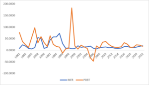
Figure 4.1: Trend of growth rate of public debt and inflation rate in Nigeria
As could be observed from Figure 4.1, the growth rate of public debt has been quite erratic over the years, with the highest growth rate of 182.46% recorded in 1999. This highest growth rate was followed by a sharp decline which reached a negative growth rate of -47.78% in 2007. One key point to note is that period of high volatility in the growth rate of public debt was matched with a greater volatility in the rate of inflation (see 1981-1998) and period of stable growth rate in public debt is matched with a stable rate of inflation (see the period 2008-2022).
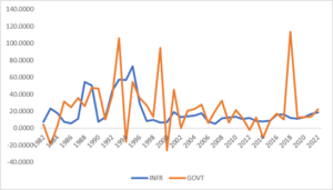
Figure 4.2: Trend of growth rate of government expenditure and inflation rate in Nigeria
The behaviour of inflation relating to the growth rate of public expenditure is reflected in Figure 4.2 and it is noticeable that the growth in government expenditure has been quite erratic over the years. In response, the rate of inflation has been highly volatile in such periods.
Descriptive Statistics
We explore the descriptive properties of the time series variables to ascertain their behaviour over the 42 years under investigation.
Table 4.1: Variables’ descriptive properties
| INFR | BRMS | INTR | TOPN | RGDP | GFCF | GOVT | PDBT | |
| Mean | 18.946 | 6.963 | 17.189 | 32.449 | 10.427 | 9.045 | 6.422 | 7.4441 |
| Median | 12.941 | 7.231 | 17.380 | 32.773 | 10.272 | 9.025 | 6.925 | 8.038 |
| Maximum | 72.835 | 10.788 | 29.800 | 62.755 | 11.235 | 9.667 | 10.103 | 10.619 |
| Minimum | 5.388 | 2.672 | 7.750 | 16.514 | 9.693 | 8.642 | 2.265 | 2.604 |
| Std. Dev. | 16.454 | 2.743 | 4.646 | 10.257 | 0.542 | 0.214 | 2.444 | 2.143 |
| Skewness | 1.877 | -0.168 | 0.307 | 0.454 | 0.225 | 0.423 | -0.352 | -0.644 |
| Kurtosis | 5.437 | 1.597 | 3.467 | 3.053 | 1.461 | 3.313 | 1.862 | 2.506 |
| Jarque-Bera | 35.057 | 3.642 | 1.044 | 1.451 | 4.499 | 1.428 | 3.138 | 3.329 |
| Probability | 0.000 | 0.161 | 0.593 | 0.484 | 0.105 | 0.489 | 0.208 | 0.189 |
| Observations | 42 | 42 | 42 | 42 | 42 | 42 | 42 | 42 |
Source: Researcher Computation
The result in Table 4.1 captures the descriptive properties of the variables. The rate of inflation (INFR) averaged 18.95% over the study period and possess a standard deviation of 16.454%. Its maximum value during the study period is reported to be 72.84% while its minimum value is 5.39%. The variable is positively skewed given its skewness coefficient of 1.88, and it is leptokurtic since the coefficient of kurtosis is greater than three. Since the Jarque-Bera statistic of 35.057 is significant at the 1% level (as could be seen from p = 0.00), then the variable is not normally distributed. For the broad money supply (BRMS), it has an average growth rate of 6.96% with a standard deviation of 2.743%. It is also observed that BRMS has a maximum and minimum value of 10.79% and 2.67% respectively. The variable is seen to be negatively skewed as seen from the -0.17-skewness coefficient, and it is platykurtic as the coefficient of kurtosis being 1.597 is less than three. However, the insignificance of the Jarque-Bera statistic confirms that the variable is normally distributed.
Interest rate (INTR) has a mean value of 17.19% with a standard deviation of 4.65% and has a maximum and minimum value of 29.80% and 7.75% respectively. The variable is positively skewed as exhibited by skewness coefficient of +0.307 and is leptokurtic given that the coefficient of kurtosis being 3.467 is greater than three. The Jarque-Bera statistic of 1.044 is statistically insignificant at the 5% level, portraying that the variable is normally distributed. Trade openness (TOPN) has an average value of 32.45% with a standard deviation of 10.26 while its minimum and maximum values were respectively 16.51% and 62.76% respectively. Trade openness is positively skewed as observed from the skewness coefficient being +0.454, and since its coefficient of kurtosis is +3.053, the distribution is almost platykurtic. Trade
openness is observed further to be normally distributed since the Jarque-Bera statistic of 1.451 is not statistically significant at the 5% level.
Another key variable of interest is the real GDP (RGDP) which is observed to have a mean value of 10.43% and a standard deviation of 0.54 and having a maximum and minimum value of 11.24% and 9.69% respectively. The variable is positively skewed given the coefficient of skewness being +0.225 and is platykurtic since 1.461 being the coefficient of kurtosis is less than three. As the Jarque-Bera statistic is insignificant, the variable is therefore characterised as being normally distributed. Gross fixed capital formation (GFCF) averaged 9.045% with a standard deviation of 0.21 and has a minimum value of 8.64% and a maximum value of 9.67%. The variable is positively skewed and leptokurtic, and it is normally distributed. In the same vein, government expenditure (GOVT) averaged 6.42% with a standard deviation of 2.44 and has a minimum and maximum value of 2.27% and 10.10% respectively. it is negatively skewed and platykurtic in nature as well as being normally distributed. Finally, public debt (PDBT) averaged 7.44% with a standard deviation of 2.14 and the variable possesses a minimum and maximum value of 2.60% and 10.62% respectively. The variable is negatively skewed, platykurtic, and normally distributed.
Correlation Analysis
The correlation analysis is conducted to check on the nature of the association among the variables of interest. It also gives an idea of whether there is any form of multicollinearity that may exist in the regression result. Table 4.2 presents the correlation matrix for the variables under consideration.
Table 4.2: Correlation Matrix
| INFR | BRMS | INTR | TOPN | RGDP | GFCF | GOVT | PDBT | |
| INFR | 1 | |||||||
| BRMS | -0.308 | 1 | ||||||
| INTR | 0.332 | 0.025 | 1 | |||||
| TOPN | 0.403 | -0.135 | 0.433 | 1 | ||||
| RGDP | -0.339 | 0.971 | -0.060 | -0.275 | 1 | |||
| GFCF | -0.296 | 0.412 | -0.383 | -0.328 | 0.498 | 1 | ||
| GOVT | -0.285 | 0.989 | 0.082 | -0.057 | 0.940 | 0.385 | 1 | |
| PDBT | -0.186 | 0.948 | 0.234 | 0.004 | 0.878 | 0.252 | 0.971 | 1 |
Source: Researcher Computation
Consistent with Table 4.2, inflation correlates negatively with public debt and public expenditure as could be seen from their respective correlation coefficient of -0.285 and -0.186. Meanwhile, this correlation coefficient is weak and portrays that such association is not a strong one. However, this does not in any way imply that there is no cause-effect relation between inflation and public debt as well as with public expenditure. Such a cause-effect relationship will be explored later in subsequent section. The explanatory variables are observed to exhibit a perfect linear relationship with each other which is an indication that the possibility of multicollinearity is very unlikely.
Unit Root Test
The unit root test is conducted to ascertain the order of integration of the variables used in the study, since they are time series in nature. Table 4.3 captures the test result which is conducted based on the augmented Dickey-Fuller (ADF) and the Phillip-Perron (PP) approaches.
Table 4.3: The unit root test result
| Augmented Dickey Fuller | Phillip-Perron | ||||||
| Variables | Level | First Difference | Order of Integration | Variables | Level | First Difference | Order of Integration |
| INFR | -4.1301 | ——– | 1(0) | INFR | -2.9662 | -10.8289 | I(1) |
| BRMS | -0.1496 | -4.3026 | I(1) | BRMS | -0.7965 | -4.2713 | I(1) |
| GCEX | -1.7655 | -6.0944 | I(1) | GCEX | -1.8535 | -6.0944 | I(1) |
| GREX | -1.8256 | -8.5885 | I(1) | GREX | -1.6003 | -8.6601 | I(1) |
| INTR | -3.3290 | -6.4943 | I(1) | INTR | -3.2192 | -10.3313 | I(1) |
| TOPN | -2.4345 | -7.6697 | I(1) | TOPN | -2.2998 | -8.3029 | I(1) |
| RGDP | -1.9703 | -3.9361 | 1(1) | RGDP | -3.0027 | -3.7921 | I(1) |
| GFCF | -7.0986 | ——- | I(0) | GFCF | -5.234 | ——– | I(0) |
| GOVT | -1.1325 | -7.7787 | I(1) | GOVT | -1.5391 | -7.6965 | I(1) |
| PDBT | -2.1971 | -4.7193 | I(1) | PDBT | -2.3743 | -4.7224 | I(1) |
| PDDT | -1.6369 | -4.9771 | I(1) | PDDT | -1.5015 | -4.9668 | I(1) |
| PEDT | -1.9848 | -4.8441 | I(1) | PEDT | -2.5916 | -4.8441 | I(1) |
Source: Researcher Computation
As could be observed from Table 4.3, the ADF unit root test result indicates that inflation rate (INFR) and gross fixed capital formation (GFCF) are stationary at level (that is, they are I(0) series) while every other variables are stationary at first difference (that is, they are I(1) series). Meanwhile, the Phillip-Perron (PP) test reported only GFCF as being stationary at level while every other variable is stationary at first difference. Since the PP approach is regarded as being more powerful than the ADF approach, the result from the PP test is being upheld.
Autoregressive Distributed Lag Model
The unit root test analysis has reported the fact that while some variables are stationary at level, others are stationary at first difference. This nature of stationarity so reported requires the use of the autoregressive distributed lag (ARDL) model in the estimation. However, the estimation starts with determination of a long-run relationship among the variables in the two models.
Bounds Test
The ARDL Bounds test for cointegration is utilized to establish the existence/non-existence of long run relationship in the models. This test is conducted for both the non-disaggregated and disaggregated model. The results are presented subsequently. It is expected that for cointegration to exists, the F-statistic must be greater than the lower and upper bounds 5% critical values.
Table 4.4: Bounds Test Result in the Non-Disaggregated Public Debt-Inflation Model
| F-Bounds Test | Null Hypothesis: No levels relationship | |||
| Test Statistic | Value | Significance | I(0) | I(1) |
| F-statistic | 4.5832 | 10% | 1.99 | 2.94 |
| K | 6 | 5% | 2.27 | 3.28 |
| 2.5% | 2.55 | 3.61 | ||
| 1% | 2.88 | 3.99 | ||
Source: Researcher Computation
It can be inferred from Table 4.4 that the F-statistic being 4.5832 lies outside the 5% lower bound (2.27) and upper bound (3.28) values. Consequently, the null hypothesis is rejected hence, there is cointegration in the model.
Table 4.5: Bounds Test Result in the Non-Disaggregated Government Expenditure-Inflation Model
| F-Bounds Test | Null Hypothesis: No levels relationship | |||
| Test Statistic | Value | Significance | I(0) | I(1) |
| F-statistic | 5.0130 | 10% | 1.99 | 2.94 |
| K | 6 | 5% | 2.27 | 3.28 |
| 2.5% | 2.55 | 3.61 | ||
| 1% | 2.88 | 3.99 | ||
Source: Researcher Computation
In line with Table 4.5, the F-statistic being 5.0130 lies outside the 5% critical lower bound (2.27) and upper bound (3.28) values hence, the null hypothesis is overruled, and we conclude that cointegration exists.
Short Run Error Correction Model
The result from the cointegration analysis presents evidence of long run relationship among variables in the models. Consequently, we explore both the short-run and long-run models. Starting with the short-run model, the results are presented subsequently.
Table 4.8: Short Run Error Correction Model for the public debt-inflation relationship
| Dependent Variable: D(INFR) | ||||
| Selected Model: ARDL(1, 3, 2, 3, 1, 2, 3) | ||||
| Variable | Coefficient | Std. Error | t-Statistic | Probability |
| D(PDBT) | -7.1778 | 7.5613 | -0.9493 | 0.3558 |
| D(PDBT(-1)) | 34.9594 | 8.1998 | 4.2634 | 0.0005** |
| D(PDBT(-2)) | 20.6761 | 6.9721 | 2.9655 | 0.0087* |
| D(BRMS) | 63.2481 | 13.5156 | 4.6796 | 0.0002** |
| D(BRMS(-1)) | 53.5153 | 16.9527 | 3.1567 | 0.0058* |
| D(INTR) | -0.9844 | 0.6196 | -1.5887 | 0.1305 |
| D(INTR(-1)) | -3.1865 | 0.7574 | -4.2074 | 0.0006* |
| D(INTR(-2)) | -3.2804 | 0.5346 | -6.1367 | 0.0000** |
| D(TOPN) | -0.7240 | 0.2816 | -2.5710 | 0.0198* |
| D(RGDP) | -48.2262 | 51.1454 | -0.9429 | 0.3589 |
| D(RGDP(-1)) | -111.5943 | 44.1627 | -2.5269 | 0.0217* |
| D(GFCF) | 7.9650 | 15.4218 | 0.5165 | 0.6122 |
| D(GFCF(-1)) | 30.9296 | 12.7608 | 2.4238 | 0.0268* |
| D(GFCF(-2)) | 23.7390 | 11.7645 | 2.0178 | 0.0597 |
| ECM(t-1) | -0.2325 | 0.0323 | -7.1946 | 0.0000** |
| R-squared | 0.7944 | Mean dependent var | -0.1119 | |
| Adjusted R-squared | 0.6745 | S.D. dependent var | 14.6304 | |
| S.E. of regression | 8.3469 | Akaike info criterion | 7.3654 | |
| Sum squared resid | 1672.0990 | Schwarz criterion | 8.0052 | |
| Log likelihood | -128.6249 | Hannan-Quinn criterion. | 7.5949 | |
| Durbin-Watson stat | 1.9192 | |||
Note: * and ** portrays significance at 5% and 1% level respectively.
Source: Researcher Computation
The result in Table 4.8 indicates that the error correction mechanism being -0.2325 is significant and negative as required, implying that the model can adjust to long run equilibrium. The coefficient signifies that 23.25% of the short run distortions in the model is corrected annually in order to restore long run equilibrium. The R-squared value of 0.7944 implies that 79.44% of the overall changes in inflation is explained by the variations in the explanatory variables. The Durbin-Watson statistic of 1.9192 (which is approximately 2), signifies the fact that the model is free from serial correlation. .
With regards to changes in broad money supply, the effect on inflation is seen to be positive and significant at the 5% level. Its one-period lag is also observed to put forth a positive and significant effect on the rate of inflation as well. The positive effect of broad money supply and its one-period lag on inflation is an indication that an increasing money supply will be associated with an increased level of inflation as postulated in the Fisher’s Quantity Theory of Money. The coefficient indicates that a 1% increase in BRMS will lead to a 63.23% increase in inflation and the one-period lag on BRMS increases the current rate of inflation by 53.52% on the average.
Changes in interest rate and its lags are observed to put forth a negative and significant influence on the rate of inflation during the period of review. This means that increasing the rate of interest will lead to a reduced rate of inflation. This is in line with the fact that an increased rate of interest (a contractionary monetary policy) will reduce the volume of money in circulation which will hitherto curb inflationary pressures within the economy. As could be noted from the coefficient, a 1% increase in INTR will lead to 0.98% decrease in inflation while the one-period and two-period lags will lead to a 3.19% and 3.28% decrease in the rate of inflation on the average.
Changes in trade openness is observed to exert a negative and significant short run effect on inflation. Thus, increased level of trade openness will be associated with a reduced level of
domestic general price level. the coefficient so obtained portrays that a 1% increase in trade openness will lead to a 0.72% decline in the general price level.
The changes in output growth is observed to exert a negative but insignificant effect on inflation while its one-period lag exerts a negative and significant effect. This is an indication that increased output growth will stall demand-pull inflation and reduce the general price level. The one-period lag of RGDP is noted to be associated with a 111.59% decline in the rate of inflation. The changes in gross fixed capital formation (GFCF) along with its lags are observed to exert a positive effect on inflation. Meanwhile, only its first-period lag exerts a significant effect by increasing the rate of inflation by 30.93% on the average. This is an indication that the existing capital stock does not support adequate domestic productivity which could curb inflation.
Table 4.9: Short Run Error Correction Model for the government expenditure-inflation relationship
| Dependent Variable: D(INFR) | |||||
| Selected Model: ARDL(2, 0, 3, 2, 3, 3, 3) | |||||
| Variable | Coefficient | Std. Error | t-Statistic | Probability | |
| D(INFR(-1)) | 0.6070 | 0.1314 | 4.6206 | 0.0003** | |
| D(GOVT) | -34.0297 | 8.2075 | -4.1462 | 0.0008** | |
| D(GOVT(-1)) | -0.8359 | 7.2101 | -0.1159 | 0.9091 | |
| D(GOVT(-2)) | 13.6589 | 6.8057 | 2.0070 | 0.0620 | |
| D(INTR) | -0.3929 | 0.5297 | -0.7418 | 0.4690 | |
| D(INTR(-1)) | -3.1473 | 0.7513 | -4.1891 | 0.0007** | |
| D(INTR(-2)) | -2.7942 | 0.6189 | -4.5148 | 0.0004** | |
| D(TOPN) | 0.2591 | 0.2821 | 0.9187 | 0.3719 | |
| D(TOPN(-1)) | 0.6051 | 0.2730 | 2.2161 | 0.0415* | |
| D(RGDP) | -102.7049 | 47.8800 | -2.1450 | 0.0476* | |
| D(RGDP(-1)) | -32.4146 | 55.0089 | -0.5893 | 0.5639 | |
| D(RGDP(-2)) | -180.6473 | 55.5408 | -3.2525 | 0.0050* | |
| D(GFCF) | -9.9380 | 15.0168 | -0.6618 | 0.5175 | |
| D(GFCF(-1)) | 59.7961 | 17.6907 | 3.3801 | 0.0038* | |
| D(GFCF(-2)) | 32.8979 | 11.9240 | 2.7590 | 0.0140* | |
| ECM(t-1) | -0.9166 | 0.1207 | -7.5927 | 0.0000** | |
| R-squared | 0.8045 | Mean dependent var | -0.1119 | ||
| Adjusted R-squared | 0.6770 | S.D. dependent var | 14.6304 | ||
| S.E. of regression | 8.3149 | Akaike info criterion | 7.3664 | ||
| Sum squared residual | 1590.1640 | Schwarz criterion | 8.0489 | ||
| Log likelihood | -127.6452 | Hannan-Quinn criterion. | 7.6113 | ||
| Durbin-Watson stat | 2.1668 | ||||
Note: * and ** portrays significance at 5% and 1% level respectively.
Source: Researcher Computation
The result in Table 4.9 presents the short-run result of the government expenditure-inflation model. The result indicates that government expenditure and its first-period lag exert a negative effect. Meanwhile, the second-period lag exerts a positive but insignificant effect. The result indicates that increasing public expenditure does not increase inflation. This finding aligns with the Critical Limit Hypothesis where if the share of government to total economic activities exceed 25%, inflation will occur even under a balanced budget. As could be seen from the coefficient, a 1% increase in government expenditure will lead to a 34.03% decrease in inflation. The error correction term indicates that the short run model adjusts by 91.66% every year in order to attain long run equilibrium. Also, the explanatory variables explain 80.48% of the entire changes in inflation as captured by the R-squared.
Table 4.10: Short Run Error Correction Model for the disaggregated public debt-inflation relationship
| Dependent Variable: D(INFR) | ||||
| Selected Model: ARDL(1, 3, 3, 2, 3, 3, 0, 3) | ||||
| Variable | Coefficient | Std. Error | t-Statistic | Probability |
| D(PDDT) | -33.2334 | 9.4309 | -3.5239 | 0.0037** |
| D(PDDT(-1)) | 77.1758 | 11.1858 | 6.8995 | 0.0000** |
| D(PDDT(-2)) | 31.0411 | 12.3267 | 2.5182 | 0.0257* |
| D(PEDT) | 8.7252 | 3.5244 | 2.4756 | 0.0278* |
| D(PEDT(-1)) | 5.7105 | 3.6775 | 1.5528 | 0.1445 |
| D(PEDT(-2)) | 16.7245 | 3.3123 | 5.0492 | 0.0002** |
| D(BRMS) | 61.2700 | 11.1471 | 5.4965 | 0.0001** |
| D(BRMS(-1)) | 32.6763 | 12.0426 | 2.7134 | 0.0177* |
| D(INTR) | -2.9548 | 0.4872 | -6.0649 | 0.0000** |
| D(INTR(-1)) | -4.6231 | 0.5647 | -8.1869 | 0.0000** |
| D(INTR(-2)) | -4.9977 | 0.5190 | -9.6293 | 0.0000** |
| D(TOPN) | -1.1478 | 0.2433 | -4.7173 | 0.0004** |
| D(TOPN(-1)) | 0.6496 | 0.2269 | 2.8626 | 0.0133* |
| D(TOPN(-2)) | -0.4323 | 0.1905 | -2.2686 | 0.0410* |
| D(GFCF) | 50.3523 | 13.3660 | 3.7672 | 0.0023* |
| D(GFCF(-1)) | 66.8601 | 11.5755 | 5.7760 | 0.0001** |
| D(GFCF(-2)) | 49.3331 | 9.9293 | 4.9684 | 0.0003** |
| ECM(t-1) | -0.3357 | 0.0330 | -10.1715 | 0.0000** |
| R-squared | 0.9019 | Mean dependent var | -0.1119 | |
| Adjusted R-squared | 0.8225 | S.D. dependent var | 14.6304 | |
| S.E. of regression | 6.1633 | Akaike info criterion | 6.7791 | |
| Sum squared resid | 797.7114 | Schwarz criterion | 7.5469 | |
| Log likelihood | -114.1932 | Hannan-Quinn criter. | 7.0546 | |
| Durbin-Watson stat | 2.2744 | |||
Note: * and ** portrays significance at 5% and 1% level respectively.
Source: Researcher Computation
For the disaggregated model where, public debt is split into domestic debt and external debt, the result indicates that changes in public domestic debt exerts a negative and significant effect on inflation. However, the first period and second-period lags are observed to exert a positive and significant effect on the rate of inflation. Thus, increased domestic debt will lead to a reduced level of inflation since it is a way of taking away liquidity from the hands of the general public, to be channelled to more productive public project. The positive effect of the lags can be attributed to the fact that such resources could be reintroduced into the monetary stream over time through public expenditure which could hitherto increase the money supply with its attendant effect on the level of domestic prices. From the coefficient, a 1% increase in public domestic debt will lead to a 33.23% decrease in the current rate of inflation. On the contrary, the first period and second-period lags of public domestic debt increased the current rate of inflation by 77.18% and 31.04% on the average.
For the public external debt, both its current value and the lags are observed to exert a positive effect on the current rate of inflation. This is an indication that external borrowings are detrimental to the domestic price level as it expands the expenditure of the government which is financed through external sources. A 1% increase in public external debt is associated with an 8.73% increase in level of inflation. Similarly, the second period lag of public external debt is observed to increase the current rate of inflation by 16.72% on the average. The error correction term indicates that 33.57% of the short run distortions in the model is corrected on a yearly basis to bring about equilibrium in the long run. The explanatory variables account for 90.19% of the total changes in the rate of inflation during the study period.
Table 4.11: Short Run Error Correction Model for the disaggregated government expenditure-inflation relationship
| Dependent Variable: D(INFR) | |||||
| Selected Model: ARDL(1, 2, 3, 1, 3, 3, 3, 0) | |||||
| Variable | Coefficient | Std. Error | t-Statistic | Probability | |
| D(GCEX) | -10.7055 | 4.0547 | -2.6403 | 0.0185 | |
| D(GCEX(-1)) | -10.2529 | 4.3794 | -2.3411 | 0.0334 | |
| D(GREX) | 2.4602 | 7.4708 | 0.3293 | 0.7465 | |
| D(GREX(-1)) | 46.3405 | 8.0005 | 5.7922 | 0.0000 | |
| D(GREX(-2)) | 34.0809 | 7.1584 | 4.7610 | 0.0003 | |
| D(BRMS) | 44.9277 | 10.4204 | 4.3115 | 0.0006 | |
| D(INTR) | 1.0083 | 0.4008 | 2.5155 | 0.0238 | |
| D(INTR(-1)) | -3.3623 | 0.6731 | -4.9955 | 0.0002 | |
| D(INTR(-2)) | -3.9767 | 0.5820 | -6.8329 | 0.0000 | |
| D(TOPN) | 0.1654 | 0.2612 | 0.6332 | 0.5361 | |
| D(TOPN(-1)) | -0.3635 | 0.2676 | -1.3585 | 0.1944 | |
| D(TOPN(-2)) | -0.8339 | 0.3003 | -2.7770 | 0.0141 | |
| D(RGDP) | 24.1643 | 47.2308 | 0.5116 | 0.6164 | |
| D(RGDP(-1)) | 68.8715 | 40.0484 | 1.7197 | 0.1060 | |
| D(RGDP(-2)) | -146.4174 | 38.7950 | -3.7741 | 0.0018 | |
| ECM(t-1) | -0.3890 | 0.0563 | -6.9112 | 0.0000 | |
| R-squared | 0.8510 | Mean dependent var | -0.1119 | ||
| Adjusted R-squared | 0.7538 | S.D. dependent var | 14.6304 | ||
| S.E. of regression | 7.2595 | Akaike info criterion | 7.0949 | ||
| Sum squared resid | 1212.1050 | Schwarz criterion | 7.7774 | ||
| Log likelihood | -122.3514 | Hannan-Quinn criter. | 7.3398 | ||
| Durbin-Watson stat | 2.1427 | ||||
Note: * and ** portrays significance at 5% and 1% level respectively.
Source: Researcher Computation
The regression result presented in Table 4.11 presents the disaggregated short run result for the government expenditure-inflation relationship. The result portrays that changes in government capital expenditure and its first-period lag put forth a negative and significant effect on inflation. This implies that capital expenditure aids in reducing the level of inflation as it enhances the capital stock which propels productivity. The coefficient indicates that a 1% increase in changes in government capital expenditure will lead to a 10.71% decrease in inflation in the short run. Also, the first-period lag of government capital expenditure reduces the current rate of inflation by 10.25% on the average. For the recurrent expenditure, its effect and that of its lags are observed to be positive. This signifies that a rising recurrent expenditure
Long Run Result
The long run estimates of the various models are presented for all the four models estimated in the short run case.
Table 4.12: Long Run Model for the public debt-inflation relationship
| Variable | Coefficient | Std. Error | t-Statistic | Probability |
| PDBT | -33.8525 | 55.7165 | -0.6076 | 0.5515 |
| BRMS | 12.0396 | 48.8844 | 0.2463 | 0.8084 |
| INTR | 3.2977 | 7.5129 | 0.4389 | 0.6662 |
| TOPN | -5.8730 | 7.4428 | -0.7891 | 0.4409 |
| RGDP | -8.1937 | 137.0852 | -0.0598 | 0.9530 |
| GFCF | 54.9516 | 212.3676 | 0.2588 | 0.7989 |
| C | -228.6788 | 1910.3290 | -0.1197 | 0.9061 |
Source: Researcher Computation
The result in Table 4.12 indicates that public debt has a negative but insignificant long run effect on inflation. This is the same case with trade openness and output growth. On the other hand, money supply, interest rate, and gross fixed capital formation all exert positive but insignificant long run effect on inflation.
Table 4.13: Long Run Model for the government expenditure-inflation relationship
| Variable | Coefficient | Std. Error | t-Statistic | Probability |
| BRMS | 27.6779 | 20.0377 | 1.3813 | 0.1862 |
| INTR | 2.7585 | 1.1857 | 2.3265 | 0.0335* |
| TOPN | -0.6875 | 0.6330 | -1.0861 | 0.2935 |
| RGDP | -34.7141 | 42.7136 | -0.8127 | 0.4283 |
| GFCF | -91.5394 | 45.2204 | -2.0243 | 0.0600 |
| GOVT | -22.6159 | 15.7702 | -1.4341 | 0.1708 |
| C | 1144.4510 | 564.7337 | 2.0265 | 0.0597 |
Note: * portrays significance at 5% level.
Source: Researcher Computation
For the government expenditure-inflation relationship, the result in Table 4.13 indicates that government expenditure exerts a negative but insignificant long run effect on inflation in Nigeria. The effect of interest rate on inflation is positive and significant in the long run. A 1% increase in interest rate is associated with a 2.76% increase in the rate of inflation in the long run. However, the effect of trade openness, output growth, and gross fixed capital formation is negative but insignificant.

Figure 4.5: Cumulative Sum of Squares for disaggregated public debt-inflation relationship.
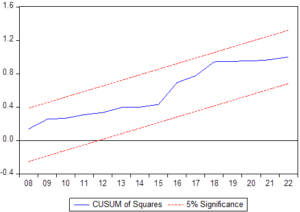
Figure 4.6: Cumulative Sum of Squares for disaggregated government expenditure-inflation relationship
As could be observed from Figure 4.3 to Figure 4.6, the CUSUM line lies within the 5% lower and upper bounds. Consequently, the stability of the parameter estimates is assured, and the parameter estimates are reliable for policy formulation.
In this study, the influence of public debt and government expenditure on inflation was being explored. The analysis covered the period 1981 to 2022 which amounts to a total of 42 years. The data for the study were obtained from the 2022 Central Bank of Nigeria statistical bulletin and the World Bank database. The specific objectives of this study were to examine the influence of public debt on inflation; to investigate the effect of government expenditure on inflation; to ascertain the threshold level of public debt that is sustainable for inflation; and to determine the threshold level of government expenditure that is sustainable for inflation. The study also embarked on both an aggregative and disaggregated analysis by disaggregating public debt into domestic and external, and disaggregating government expenditure into capital expenditure and recurrent expenditure. The study adopts the analytical technique of both the autoregressive distributed lag (ARDL) model and the threshold regression analysis. The major findings of the study are highlighted as follows:
Public debt exerts a negative but insignificant short run effect on inflation while its lags exert a positive and significant effect on inflation. This implies that the past values of public debt cause the current rate of inflation to increase. Meanwhile, the long run effect of public debt on inflation is negative but insignificant.
Government expenditure exerts a negative and significant effect on inflation in the short run, but its lags exert an insignificant effect. This implies that in the short run, increased public expenditure will not intensify inflationary pressures within the economy. The long run effect of government expenditure is observed to be negative but statistically insignificant.
By disaggregating public debt into domestic and external debt, our result indicates that changes in public domestic debt exerts a negative and significant short run effect on inflation while its lags put forth a positive and significant effect. This implies that the current level of domestic debt aids to reduce inflation while the past value of domestic debt accelerates inflationary pressures in the Nigerian economy. On the contrary, the external debt and its lags put forth positive and significant short run effect on inflation, implying that they drive inflationary pressures in the Nigerian economy. In the long run, both domestic debt and external debt exerts a negative effect on inflation though such effect is insignificant.
By disaggregating government expenditure into capital and recurrent expenditures components, the findings of the study indicated that while capital expenditure exerts negative and significant short run effect on inflation, recurrent expenditure put forth positive and significant effect. This implies that capital expenditure does not drive-up inflationary pressures but the recurrent expenditure component is inflationary in nature. In the long run, both capital and recurrent expenditure components exert negative but insignificant effect on inflation.
The threshold regression result indicated that the optimal threshold level of public debt is 17.35% while that of government spending is 15.8130%. The implication here is that above these thresholds’ levels, public debt and government spending will respectively exert positive effects on inflation, implying that they will drive up inflationary pressures after their respective threshold levels.
Given the findings, the study concludes that though public debt and government expenditure are observed to exert negative effect on inflation during the study period, it does not imply that all the components of public debt and government expenditure are not inflationary in nature. The evidence therefore portrays that only domestic debt and capital expenditure are not inflationary in nature while external debt and recurrent expenditure are highly inflationary in nature. Given this, the study presents the following recommendations:
The government, through its budget, must resort to increasing its capital expenditure component while ensuring that the recurrent expenditure component is not rapidly increased.
The government needs to resort to increased attention to borrowing within the country and less from external sources which have been found to drive up inflationary pressures in the economy.
Finally, there is need to strictly adhere to the threshold level of 17.35% for public debt and 15.8130% for government spending. Exceeding these thresholds levels have the potential to cause public debt and government expenditure to accelerate inflationary pressures in the economy.