Building a Suitable Generalized Autoregressive Conditional Heteroskedasticity Time Series Model: A Nigeria Net Migration Rate Application
Nwankwo,I.O , Nworuh, G.E and Okoli, C.N
Department of Statistics, Chukwuemeka Odumegwu Ojukwu University, Anambra State, Nigeria.
This work focused to build a Suitable Generalized Autoregressive Conditional Heteroskedasticity model for solving net migration rate problem in Nigeria. Analyzing the 51 year annual data of Net Migration Rate (NMR), Crude Death Rate (CDR), Fertility Rate (FR), Inflation Rate (IR), Real Annual Gross Domestic Product (RAGDP), Population Growth Rate (PGR) and Exchange Rate (ER) with Econometric Views (EViews) version 12.0 statistical software, the data was first represented on a graph to show a historical pattern of the variables. A multiple regression analysis was carried out to ascertain the nature of relationship existing between NMR (dependent variable) and ER, IR, CDR, PGR, FR and RAGDP as the independent variables. The results obtained showed a strong positive relationship and that the regression is not spurious. The series being Stationary was used for hypothesis testing, forecasting and fitting of time series models. With Augmented Dickey-Fuller (ADF) test, six series were stationary while with Kwiatkowski-Philips-Schmidt-Shin (KPSS) test, one was stationary. The Q-Statistics probability values were all greater than 0.5 across 36 – lags implying no ARCH models and residuals normally distributed. No autocorrelation, no heteroskedasticity and residuals normally distributed indicating that the GARCH family models studied with three error distributions can be employed to find the best model for solving migration rate problem in Nigeria. Normal Gaussian error distribution EGARCH (1, 1) performed best. The key measurable factors affecting NMR in Nigeria as observed in this work are ER, IR and PGR. Further studies should be done on both Normal Gaussian error distributions EGARCH from 2nd order, symmetric and asymmetric GARCH models to ascertain their performances in modeling Net Migration rate in Nigeria.
Keywords: Net migration rate, GARCH, Error distribution, Normal Gaussian, Durbin-Watson.
Recent economic crisis, political instability, ecological disturbances, and social crisis changed dramatically economic conditions in many countries. This contributed to the changes in the volume or even directions of migration flows within Nigeria as well as between Nigeria and other countries of the world. Several factors have been marked to have contributed to this massive movement of people. Studies indicate that the key determinants of migration include the availability of migrant networks, differences in income across countries, and demographic factors, but many other factors also affect the migration decision. Constraints created by migration policy represent the most significant hurdle to migration amidst countries of the world. Nigeria as a country in the West Africa has suffered migration problems since independence. Her migrants had several reasons to migrate. Regional crisis, insecurity, insurgency, banditry, kidnapping, communal clashes, over flooding, economic hardship, unemployment, poor wage system, poor access to quality education and health care, hike in prices of goods and services, and etc. are all identified factors peculiar with Nigeria.
Despite various attempts by researchers to explore the relationship between net migration and several factors, none seems to have attempted to fit a time series model using GARCH family models such as Fractionally integrated exponential generalized autoregressive conditional heteroskedasticity (FIEGARCH), Fractionally integrated generalized autoregressive conditional heteroskedasticity (FIGARCH), Autoregressive conditional heteroskedasticity (ARCH), Component autoregressive conditional heteroskedasticity (Component ARCH), Exponential generalized autoregressive conditional heteroskedasticity (EGARCH), Generalized autoregressive conditional heteroskedasticity (GARCH) and Power autoregressive conditional heteroskedasticity (PARCH) nor attempted to study the relationship between net migration and the unique variables of interests which includes crude death rate (CDR), exchange rate (ER), fertility rate (FR), inflation rate (IR), population growth rate(PGR) and real annual gross domestic product (RAGDP) on net migration rate (NMR) in Nigeria, hence the essence of this work.
According to Afaha (2013), Nigeria plays a crucial role in African and other parts of the world migration. He went further to opine that as the most populous African country, Nigeria has become involved in international migration in an increasing form to countries such as Europe, South Africa and Gulf countries. He noted that the economic reasons for this migration in most cases are related to wage differences, large economic disparity in regions, differences in per-capita GDP and unemployment differentials.
Abiola (2019) noted that what however that posse a great threat towards Nigeria attaining economic growth is the number of emigrants that grows significantly against that of the immigrants. Statistics put up by the World Development Indicators (2014) shows that net-migration for Nigeria in 1992 was -95,769 which rose in 2002 to 170,000 while in 2012 it was recorded to be -300,000. This however indicates that net-migration for the country is rapidly increasing and has remained negative. Furthermore, in 2016, the net – migration was -327 per thousand populations, while in 2017, it stood at -3.19 per thousand populations which shows a drop when compared to 2016 data (WDI, 2017).
Drinkwater, Lotti, Levine and Pearlman (2003) in their research assertion emphasized that migration may drain away valuable talents, given that since most educated motivated people are in most cases likely to move in search of better opportunities. They further added that about 10.7% of highly trained Nigerian skilled work force in 2000 migrated to most especially Economic Cooperation and Development (OECD) countries. Fadahunsi and Rosa (2002) said that on the average, 64% of Nigerian emigrants completed tertiary education. These however are evidence to support to the assertion that many trained professionals, athletes and other skilled work force who could have contributed to the growth and development of the country should they be engaged have abandoned the nation to other favorable nations where they use their skills to aid the development of their receiving countries.
Arango (2002) opined that workers usually move from countries with low wages and abundance of labour to scarce labour countries with higher wages. Hence the main motivation of migration is the increased welfare that individuals receive from higher labour income or wages. The neoclassical theory however is argued to suppress the role of non-economic factors which to a large extent play a deterministic role in an individual migrant’s decision to leave his home country. The theory failed to explain why few people move in view of existing large income gaps across countries. One would expect that massive movement of work force would be migrating across countries (that have scarce labour) with new information of the perception of higher returns on labour, but the reality is that existing barriers such as obtaining travel permits, visas and other documents which intending migrants must have, limit the degree of such exchange of labour across countries referred to as labour immobility.
Arango (2002) also stated the dual labour market theory as an important theory applicable to migration links immigration to the structural requirements of modern industrial societies. The theory states that international migration is largely demand based and is initiated by recruitment on the part of employers in developed societies or by government acting on their behalf; migration is driven by an increasing demand for “cheap’ labour. This theory however pays more attention to the migration receiving countries or regions. It presumes that many developed economies require immigrant workers to take up jobs, which local workers have refused.
Sanderson and Kentor (2009) findings using cross national empirical analysis to examine the relationship between globalization, development and international migration from 1970 to 2000 in less developed countries showed that there is a significant non-linear relationship between net migration and economic development.
Ramirez, Gonzalez, Martel and Agoh (2018) result of their investigation on the contribution of migration to economic growth in Spain from 2009 to 2015 using input output analysis indicated a positive relationship between migration and economic growth.
Kotani (2012) took an empirical study to understand the effect of net-migration on economic growth relations in Indonesia which he employed Ordinary Least Square (OLS) regression technique with an annual time series data (Gross domestic product, population growth, fertility rate and net migration) ranging from 1993 to 2005. The study however revealed that lagged fertility rate does not affect economic growth in the two variable regression; thus, there exists a significant negative relationship between population and economic growths upon the inclusion of net-migration as a variable in the model. He concluded therefore that net-migration is a key determinant of economic growth.
Akanbi (2017) investigated the impact of migration on economic growth and human development in sub-Saharan African countries from 1999 to 2013 using two stage least square estimation techniques for the analysis, the result showed a significant negative relationship between migration and economic growth.
Obomeghie, Abubakar and Abdurrahman (2018) investigated the impact of net migration on total fertility rate in sub-Saharan African countries using descriptive statistics method, with empirical evidence from Nigeria for the period of 2000 to 2016. They found out that net migration impact positively in Nigeria.
Afaha (2013) investigated the relationship between migration, remittances and development in Nigeria from the periods of 1977 to 2008 and employed a household survey – based method. In his study, he found out that migrant’s remittances in Nigeria had significant positive relationship with the economic growth.
Darkwah and Verter (2014) in their study examined the determinants of international migration in Nigeria from 1991 to 2011. Employing the method of Ordinary Least Square estimation, they found from their result that the level of unemployment, migrant’s remittances and population growths are the key determinants of emigration to other countries from Nigeria. Their findings also shows that there is a strong positive relationship between the numbers of Nigeria’s abroad and unemployment rate, migrant’s remittances and population growth in Nigeria.
Abiola (2019) investigated on the impact of labour migration remittances and economic growth in Nigeria from 1980 to 2016 using indirect least square approach, there is a positive relationship between emigration and economic growth in Nigeria.
Umar and Abdullahi (2019) who empirically examined the impact of net population growth and economic growth in Nigeria using a time series data from 1970 to 2017, the result using Autoregressive distributed lag (ARDL) model approach revealed a negative and significant long run co integrating relationship between economic growth and net population growth within the period of study and that a unidirectional causality exists running from net population growth to economic growth. This study however failed to address the differences between emigrants and immigrants and its relationship to economic growth.
Hsieh (1988) who first applied the ARCH model for the exchange rate concluded that indiscriminate ARCH (GARCH) model can describe single part of the nonlinearity of exchange rates.
Sandoval (2006) studied Asian and Latin American countries exchange rates with respect to the US dollar using GJR-GARCH, GARCH and EGARCH models. He discovered that out of the seven exchange rates studied, four follow asymmetric models.
Marisetty (2024) who used leading global stock indexes evaluated several GARCH models, which includes Generalized Autoregressive Conditional Heteroskedastics (GARCH), Exponential Generalized Autoregressive Conditional Heteroskedastics (EGARCH), Nonlinear Generalized Autoregressive Conditional Heteroskedastics (NGARCH), Asymmetric Power Autoregressive Conditional Heteroskedastics (APARCH), Glosten-Jagannathan-Runkle Generalized Autoregressive Conditional Heteroskedastics (GJR-GARCH) and Threshold Generalized Autoregressive Conditional Heteroskedastics (TGARCH) to forecast volatility and addresses both symmetric and asymmetric effects found out that TGARCH model exhibited strong performance in capturing leverage effects and asymmetries, particularly for FTSE 100 and Hang Seng index. The APARCH model he found out performed well for S & P 500, demonstrating sensitivity to past shocks. His findings however, underscores the significance of advanced GARCH models in correctly predicting the TGARCH model’s effectiveness in addressing asymmetries and providing insights in choosing appropriate models for enriched financial analysis and risk management.
According to Eriyeva and Okoli (2021), a comparative performance of five GARCH models ((Simplified Generalized Autoregressive Conditional Heteroskedastics (SGARCH), GJRGARCH, EGARCH, APGARCH and Integrated Generalized Autoregressive Conditional Heteroskedastics (IGARCH)) using United Bank for Africa daily stock exchange prices in Nigeria revealed that EGARCH (1,1) model performed optimally because it achieved the least AIC, indicated volatility clustering as well as leverage effects on the UBA daily stock exchange prices for the period of ten years.
Dritsaki (2018) examined the characteristics of British pound exchange rate/US dollar volatility using monthly data from August 1953 to January 2017. Employing both static and dynamic procedures to forecast the ARIMA (0, 0, 0, 1) – EGARCH (1, 1) model, the static procedure was shown to give better results on the forecast than on the dynamic procedure.
Akanbi, Olatayo and Taiwo (2025) evaluated and compared the performance of four variant of GARCH model incorporating skewed non-Gaussian error innovation distribution using daily closing prices of Bitcoin, Naira to Dollar Exchange rates and daily Nigeria all Share Index from January 1, 2015, and January, 26, 2024. The result of their studies shows that the model of GJR-GARCH (1, 1) with skewed Student-t (sstd) performed optimally for all share indexes. EGARCH (1, 1) – sstd performed well for USD-Naira while GARCH (1, 1)-sged performed good for Bitcoin. They concluded by noting the superiority of the skewed Student-t distribution in most of the cases which offers valuable insights for investors on when and how to invest their assets.
Ali (2011) who pioneered the use of ARCH and GARCH models in environmental literature used asymmetric ARCH and GARCH models to issue beach advisories for pathogen indicators. Engel (1982) developed the time varying model while Bollerslev (1986) extended the model to include the ARMA structure. Glosten, Jagannathan and Runkle (1993) introduced GARCH with differing effects of negative and positive shocks taking into account the leverage phenomenon. Alberg, Shalit and Yosef (2008) showed that the GARCH models with fat-tail distributions are relatively better suited for analyzing returns on stocks.
Odum and Okoli (2021) who carried out a study on Autoregressive Conditional Heteroscedasticit (ARCH) Modeling of the Nigerian Stock Indices using seven Distribution for Innovation revealed that out of the seven parametric distributions (Gaussian distribution, the skewed Gaussian distribution, the Student’s t distribution, the Generalized error distribution, the Skewed Generalized error distribution, the Standardized normal inverse Gaussian distribution and the Skewed Student’s t distribution ) fitted on the data using Maximum Likelihood method, the ARCH model with the Student’s t distribution outperformed other distributions suggesting it gave the best fit having considered all the selection criterion of low yield in Akaike Information Criterion (AIC), Bayesian Information Criterion (BIC) and Hannan-Quinn Information Criterion (HQC).
Nelson (1991) used Exponential distribution for the U.S. stock market returns. Hsieh (1989), Theodossiou and Koutmos (1994) used it for foreign exchange rates. Akgirary et al (1991) applied it for the price distribution of precious metal. This shows that the assumption of normal distribution has been relaxed in modeling the effect of volatility.
Gallant, Hsieh and Tauchen (1997) adopted the non – normal distribution for the financial analysis. Jun Yu (2005) Siourounis (2002) also preferred the non – normal distributing, Speight and Apgwilyn (2000) had symmetric and asymmetric densities for the United Kingdom stock market.
Fernandez and Steel (1998) used the skewed Student’s t distribution. Lambert and Laurent (2001) used it in the GARCH framework.
Baillie and Bollerslev (1989) used the Student’s t distribution to model the foreign exchange rate.
Harrris, Kucukozmen and Yilmaz (2004) used the skewed generalized Student’s t distribution to capture stylized facts (skewness and leverage effects) of daily returns.
Ding, Granger and Engle (1993) used the asymmetric power autoregressive conditional hetero (APARCH) model using standard and poor’s data.
Method of Data Collection
The data for this research were collected using the internet. As a secondary data, the source include Central Bank of Nigeria Statistical Bulletin, National Bureau of Statistics (NBS), World development report, Population reference Bureau, World data atlas Nigeria and knoema.com. The data used for this thesis includes: Net Migration Rate, Fertility Rate, Exchange Rate, Population Growth Rate, Inflation Rate, Annual Gross Domestic Product and Crude Death Rate. Each of these data was collated over a 51 year period. The problems encountered during the search and collation of the requisite data for the thesis includes poor network, inconsistency in electricity supply, high cost in the purchase of the data from certain data agency that makes merchant from their stored data and time due to other factors demanding someone’s attention and time.
Data Presentation
Research data collected from 1970 – 2020
| YEAR | FR (%) | ER (%) | RAGDP (%) | CDR (%) | IR (%) | NMR (%) | PGR (%) |
| 1970 | 6.471 | 0.7 | 25.007 | 22.810 | 13.76 | -0.149 | 2.31 |
| 1971 | 6.522 | 0.7 | 14.238 | 22.491 | 16.00 | -0.143 | 2.35 |
| 1972 | 6.575 | 0.7 | 3.364 | 21.163 | 3.46 | -0.136 | 2.39 |
| 1973 | 6.625 | 0.7 | 5.393 | 21.826 | 5.40 | -0.129 | 2.47 |
| 1974 | 6.669 | 0.6 | 11.161 | 21.480 | 12.67 | 0.377 | 2.60 |
| 1975 | 6.706 | 0.6 | -5.228 | 20.127 | 33.96 | 0.883 | 2.75 |
| 1976 | 6.735 | 0.6 | 9.042 | 20.766 | 24.30 | 1.388 | 2.91 |
| 1977 | 6.757 | 0.6 | 6.024 | 20.404 | 15.09 | 1.894 | 3.04 |
| 1978 | 6.772 | 0.6 | -5.764 | 20.050 | 21.79 | 2.400 | 3.08 |
| 1979 | 6.781 | 0.6 | 6.759 | 19.713 | 11.71 | 1.575 | 3.02 |
| 1980 | 6.783 | 0.5 | 4.205 | 19.408 | 9.97 | 0.750 | 2.89 |
| 1981 | 6.779 | 0.6 | -13.128 | 19.149 | 20.81 | -0.075 | 2.75 |
| 1982 | 6.767 | 0.7 | -6.803 | 18.943 | 7.70 | -0.900 | 2.63 |
| 1983 | 6.749 | 0.7 | -10.924 | 18.790 | 23.21 | -1.725 | 2.57 |
| 1984 | 6.726 | 0.8 | -1.116 | 18.689 | 17.82 | -1.421 | 2.56 |
Research data collected from 1970 – 2020 continues
| 1985 | 6.698 | 0.9 | 5.913 | 18.633 | 7.44 | -1.117 | 2.60 |
| 1986 | 6.664 | 1.8 | 0.061 | 18.610 | 5.72 | -0.813 | 2.64 |
| 1987 | 6.625 | 4 | 3.200 | 18.60 | 11.29 | -0.509 | 2.66 |
| 1988 | 6.582 | 4.5 | 7.334 | 18.603 | 54.51 | -0.205 | 2.67 |
| 1989 | 6.537 | 7.4 | 1.919 | 18.596 | 50.47 | -0.202 | 2.65 |
| 1990 | 6.490 | 8 | 11.777 | 18.579 | 7.36 | -0.199 | 2.61 |
| 1991 | 6.443 | 9.9 | 0.358 | 18.553 | 13.01 | -0.195 | 2.58 |
| 1992 | 6.395 | 17.3 | 4.631 | 18.524 | 44.59 | -0.192 | 2.55 |
| 1993 | 6.348 | 22.1 | -2.035 | 18.492 | 57.17 | -0.189 | 2.53 |
| 1994 | 6.303 | 22 | -1.815 | 18.454 | 57.03 | -0.184 | 2.52 |
| 1995 | 6.262 | 21.9 | -0.073 | 18.406 | 72.84 | -0.179 | 2.52 |
| 1996 | 6.224 | 21.9 | 4.196 | 18.348 | 29.27 | -0.175 | 2.52 |
| 1997 | 6.190 | 21.9 | 2.937 | 18.276 | 8.53 | -0.170 | 2.52 |
| 1998 | 6.159 | 21.9 | 2.581 | 18.182 | 10.00 | -0.165 | 2.52 |
| 1999 | 6.131 | 92.3 | 0.584 | 18.059 | 6.62 | -0.184 | 2.53 |
| 2000 | 6.106 | 101.7 | 5.016 | 17.895 | 6.93 | -0.203 | 2.54 |
| 2001 | 6.083 | 111.2 | 5.918 | 17.675 | 18.87 | -0.222 | 2.54 |
| 2002 | 6.060 | 120.6 | 15.329 | 17.397 | 12.88 | -0.241 | 2.55 |
| 2003 | 6.036 | 129.2 | 7.347 | 17.063 | 14.03 | -0.260 | 2.57 |
| 2004 | 6.011 | 132.9 | 9.251 | 16.682 | 15.00 | -0.289 | 2.59 |
| 2007 | 5.985 | 131.3 | 6.439 | 16.267 | 17.86 | -0.318 | 2.62 |
| 2006 | 5.958 | 128.7 | 6.059 | 15.836 | 8.23 | -0.346 | 2.65 |
| 2007 | 5.930 | 125.8 | 6.591 | 15.409 | 5.39 | -0.375 | 2.67 |
| 2008 | 5.902 | 118.6 | 6.764 | 15.002 | 11.58 | -0.404 | 2.69 |
| 2009 | 5.872 | 148.9 | 8.037 | 14.622 | 12.50 | -0.394 | 2.70 |
| 2010 | 5.839 | 150.9 | 8.006 | 14.270 | 13.72 | -0.384 | 2.71 |
| 2011 | 5.802 | 153.9 | 5.308 | 13.942 | 10.82 | -0.373 | 2.71 |
| 2012 | 5.758 | 157.5 | 4.230 | 13.623 | 12.22 | -0.363 | 2.72 |
| 2013 | 5.709 | 157.3 | 6.671 | 13.307 | 8.48 | -0.353 | 2.71 |
| 2014 | 5.653 | 158.6 | 6.310 | 12.994 | 8.06 | -0.344 | 2.70 |
| 2015 | 5.592 | 192.4 | 2.653 | 12.686 | 9.01 | -0.336 | 2.68 |
| 2016 | 5.526 | 253.5 | -1.617 | 12.390 | 15.68 | -0.327 | 2.66 |
| 2017 | 5.457 | 305.8 | 0.806 | 12.114 | 16.52 | -0.319 | 2.64 |
| 2018 | 5.387 | 306.1 | 1.923 | 11.860 | 12.09 | -0.310 | 2.62 |
| 2019 | 5.317 | 306.9 | 2.208 | 11.630 | 11.40 | -0.303 | 2.60 |
| 2020 | 5.420 | 358.8 | -1.794 | 11.420 | 33.30 | -0.295 | 2.58 |
Table 3.3 contains all the data for this work collected over a 51 year period (1970 – 2020).
Graphical Presentation and Interpretations
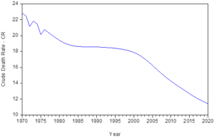
Figure 4.1: Crude Death Rate in Nigeria from 1970 – 2020
Figure 4.1 is the graphical representation of Crude Death Rate in Nigeria from 1970 to 2020. The graph generally shows a downward pattern of movement to the right.
Observing from 1970, Nigeria recorded a high death rate which was followed by a low death rate until 1973 when the death rate rose to 21.826%. This however could be attributed to the effect of civil war, increased poverty and hunger, lack of basic amenities to sustain life together with the fact that Nigeria as a Nation was still struggling to set her feet strong on the ground since independence.
The rise and fall in Nigeria’s Crude death rate continued up till 1976 when it experienced another sharp increase from 20.127% in 1975 to 20.766% in 1976 after which it maintained a wavelike smooth downward trend pattern up to year 2020. This could however be attributed to the fact that Nigeria as a Nation having survived the impact of Nigeria-Biafra war especially on her population and economic activities, greatly worked to improve the health and life of her citizens by providing basic life sustaining programs and facilities which were not there in the first place such as Operation Feed the Nation OFN in 1977, NEEDS, the green revolution of 1980, Directorate of Foods, Roads and Rural infrastructure (DFFRI), the National Directorate for Employment (NDE), Poverty Alleviation Programs (PAP), National Poverty Eradication program (NAPEP), Teaching Hospitals and Special Medical Centers, NHIS, and etc.
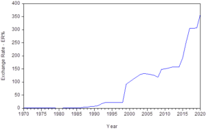
Figure 4.2: Exchange Rate in Nigeria from 1970 – 2020
We observe from figure 4.2 that Nigeria Exchange Rate maintained a steady flat movement along the vertical axis representing the year from 1970 to 1985. It however began rising from 1986 to 1994 when it maintained a continuous flat rate for the period of four (4) years (1995 to 1998). At 1999, it had a sharp increase far above 50%and never came below 50% as the year comes.
Since it had a sharp increase in 1999, the Exchange Rates been increasing in a tremendous manner without any hope of it coming down as obtained from 1970 to 1990. This however could be attributed to the decline in the oil boom in Nigeria in 1995 which deeply affected her economy as she solely depended on crude oil since its discovery with much prospects from 1989, abandoning her Agricultural product on which she has largely survived with great comparative advantage.

Figure 4.3: Fertility Rate in Nigeria from 1970 – 2020
Figure 4.3 represents the Fertility Rate in Nigeria from 1970 to 2020. Observing the graph closely, we saw that Fertility Rate in Nigeria increased rapidly from 6.471% in 1970 to 6.783% in 1980 which is the year with the highest Fertility Rate probably since her independence.
Shortly after the peak of her Fertility Rate in 1980, Nigeria as a Nation has maintained a decreasing Fertility Rate from 6.779% in 1981 to 5.317% in 2019 after which it had a sharp increase to 5.420% in 2020.
Nigeria struggling with her Fertility Rate between 1970 and 1980 indicates a country faced with population boom void of requisite programs and campaigns aimed at minimizing her fertility rate. This challenge however made her to lunch into massive programs such mass literacy, etc. it has also possibly been influenced negatively by the rise in poor economic conditions as seen in exchange rate. People now learnt to give birth to few children the can comfortably cater for in their homes.
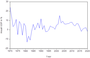
Figure 4.3: Real Annual Gross Domestic Product of Nigeria from 1970 – 2020
Figure 4.3 shows the Real Annual Gross Domestic Product of Nigeria from year 1970 to year 2020. This however is the sum of the gross value added by all resident producers in the economy plus any product taxes and minus any subsidies not included in the value of the products.
Taking a close look at the graph, we observed that over the 51 year period, period of low RAGDP were followed by periods of high RAGDP. It kept fluctuating over the entire period of the study with 1970 recording highest value of 25.007%.
The two other years with vivid increase in the RAGDP include 1990 (11.777%) and 2002 (15.329%). The year with the least RAGDP was 1981 which recorded a negative value of (-13.128%) followed by 1983 with the value of (-10.924%). Out of the 51year period of the study, only 11 years had an Annual Real GDP fall below 0.00% while others had value above 0.00%.
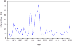
Figure 4.5: Inflation Rate in Nigeria from 1970 – 2020
Figure 4.5 shows the graphical representation of the Inflation Rate in Nigeria from 1970 to 2020. The graph generally shows a high fluctuating pattern over the 51year period of the study. The periods of high inflation rate is followed by the periods of low inflation rate and the periods of low inflation rate is followed by the periods of high inflation rate.
In 1970, Nigeria had her inflation rate increased from 13.76% to 16.00% in 1971 with a sharp drop in 1972 after which there was a great rise to above 30% in 1975. Its fluctuation continued until 1988 when it raised to 54.51%, dropped again in 1990 to 7.36% with a continued fluctuation and by 1995 (the year oil boom in Nigeria dropped greatly), the worst inflation rate hit Nigeria with a value of 72.84%. Though it dropped two years after, it however continued in its fluctuation pattern until 2020 when a notable and sharp increase to 33.30% was observed.
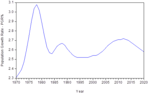
Figure 4.6: Population Growth Rate in Nigeria from 1970 – 2020
Figure 4.6 is the graphical representation of the rate of Population Growth in Nigeria from 1970 to 2020. The graph however shows a sinusoidal pattern of growth. A period of increase follows a period of decrease and a period of decrease follows a period of increase.
The PGR in the country rose from 2.31% in 1970 to 3.08% in 1978 after which there was a decrease from 3.08% in 1978 to 2.56% in 1984. It increased however for a period of four (4) years as obtained from 1985 (2.60%) to 2.67% in 1988. Another increase in the rate of growth in Nigeria’s population happened between 1989 and 1993.
Moving away from 1993, the country had a steady growth rate of 2.52% for a stretch period of five (5) years that is from 1994 to 1998 from which the country began experiencing rapid growth in her population for a good period of 14 years that is from 1999 to 2012 with a decrease which continued from 2013 to 2020.
In all the 51% year period of the study, Nigeria’s Population had its highest peak in 1978 and its lowest peak in 1970 followed by the periods between 1993 and 1998.
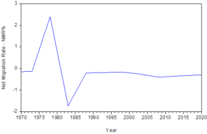
Figure 4.7: Net Migration Rate in Nigeria from 1970 – 2020
Figure 4.7 shows the graphical representation of Net Migration in Nigeria from 1970 to 2020
Nigeria’s Net Migration rate maintained a stable growth of -0.1% in 1970 to 0.379 in 1974 when a notable position increase was made. Between 1974 and 1978 (4 years apart), Nigeria had a steady increase in her Net Migration Rate with 1978 as the worst hit characterized by people moving to find greener pastures in the city areas and across the countries boarder. Thereafter, there was a sharp drop in the rate on migration in the country from 2.400% in 1970 to -1.725% in 1983 though it had a noticeable negative increase from -1.725% in 1983 to -0.205% in 1988 after which it maintained a steady but slow decreasing rate till 2020.
Regression Analysis and Interpretations
Table 4.1: Showing Regression Analysis output using EVIEW 12.0 version
Dependent Variable: NET MIGRATION RATE
Method: Least Squares
Date: 02/21/22 Time: 22:56
Sample: 1970 2020
Included observations: 51
| Variable | Coefficient | Std.Error | t-Statistics | Prob. |
| C | -6826734 | 1.373430 | -4.970573 | 0.0000 |
| Crude Death Rate | 0.526319 | 0.036235 | 14.52527 | 0.0000 |
| Exchange Rate | 0.001988 | 0.000972 | 2.044022 | 0.0470 |
| Fertility Rate | -2.700594 | 0.297409 | -9.080409 | 0.0000 |
| Inflation Rate | 0.005740 | 0.002004 | 2.864606 | 0.0064 |
| Population Growth Rate | 5.372242 | 0.253875 | 21.16100 | 0.0000 |
| Real Annual GDP | -0.012453 | 0.006045 | -2.059997 | 0.0453 |
| R-squared | 0.925337 | Mean dependent var | -0.134275 | |
| Adjusted R-squared | 0.915156 | S.D dependent var | 0.707562 | |
| S.E. of regression | 0.206099 | Akaike info criterion | -0.194045 | |
| Sum squared resid | 1.868981 | Schwarz criterion | 0.071107 | |
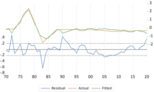
Figure 4.8: The Residual Plot
Figure 4.8 is the graphical plot of the residual distribution from 1970 to 2020. We however observed that periods of high net migration is followed by the period of low net migration in a fluctuating manner from 1970 to 1978. Periods of high net migration is followed by a prolonged period of low net migration between 1978 and 1989 while period of low net migration is followed by a prolonged period of low net migration from 1990 to 2020.
Table 4.2: Table showing Data Stationarity using ADF and KPSS at 5% level of significance
| Variable | Test type | Data Type | Intercept | Trend &
Intercept |
Test type
value |
t-Statistic | p-value | Decision |
| CDR | ADF | 2nd DIFFERENCE | NO | YES | -4.618726 | -3.540328 | 0.0038 | Stationary |
| ER | ADF | 2nd DIFFERENCE | NO | YES | -7.373165 | -3.526609 | 0.0000 | Stationary |
| FR | KPSS | 2nd DIFFERENCE | YES
|
NO
|
0.321792
|
0.463000
|
N/A
|
Stationary
|
| IR | ADF | LEVEL | NO | YES | -3.501002 | -2.921175 | 0.0120 | Stationary |
| NMR | ADF | LEVEL | YES | NO | -4.487145 | -2.936942 | 0.0009 | Stationary |
| PGR | ADF | LEVEL | YES | NO | -3.645115 | -2.929734 | 0.0086 | Stationary |
| RGPD | ADF | LEVEL | YES | NO | -5.611919 | -2.921175 | 0.0000 | Stationary |
From table 4.2, we observed that the series became stationary with ADF and KPSS tests. With ADF test, the inflation rate, net migration rate, population growth rate and real annual gross domestic product series became stationary at the level data type with the absolute values of the test type greater than their corresponding absolute t-statistics values which are all significant having considered their corresponding p-values which are each greater than 0.05 as obtained in table 4.2. The crude death rate and exchange rate series were also observed to be stationary with ADF test but at 2nd difference data type respectively. The corresponding p-values which are less than 0.05, shows that their test values are significant and that the absolute values of the test type are each greater than their t-statistic values.
Table 4.3: Q-Statistics Probability values distributed across the GARCH family models with their respective Error Distributions
| s/ n | GARCH (1,1)
|
EGARCH (1,1) | ARCH (1) | Comp. ARCH (1,1) | FIGARCH | FIEGARCH | PARCH (1,1) | |||||||||||||
| N | S | G | N | S | G | N | S | G | N | S | G | N | S | G | S | G | N | S | G | |
| 1 | 0.990 | 0.810 | 0.722 | 0.295 | 0.601 | 0.580 | 0.567 | 0.693 | 0.775 | 0.811 | 0.658 | 0.641 | 0.058 | 0.545 | 0.296 | 0.282 | 0.743 | 0.577 | 0.721 | 0.531 |
| 2 | 0.604 | 0.588 | 0.501 | 0.527 | 0.816 | 0.851 | 0.726 | 0.825 | 0.840 | 0.969 | 0.875 | 0.864 | 0.153 | 0.749 | 0.452 | 0.424 | 0.946 | 0.527 | 0.540 | 0.438 |
| 3 | 0.591 | 0.458 | 0.412 | 0.535 | 0.910 | 0.748 | 0.578 | 0.730 | 0.740 | 0.835 | 0.719 | 0.673 | 0.145 | 0.624 | 0.558 | 0.187 | 0.533 | 0.437 | 0.387 | 0.347 |
| 4 | 0.651 | 0.496 | 0.452 | 0.318 | 0.837 | 0.797 | 0.567 | 0.752 | 0.755 | 0.665 | 0.668 | 0.604 | 0.147 | 0.564 | 0.594 | 0.260 | 0.443 | 0.451 | 0.379 | 0.369 |
| 5 | 0.713 | 0.589 | 0.556 | 0.392 | 0.917 | 0.877 | 0.590 | 0.828 | 0.832 | 0.782 | 0.778 | 0.729 | 0.157 | 0.643 | 0.701 | 0.367 | 0.391 | 0.520 | 0.464 | 0.457 |
| 6 | 0.763 | 0.679 | 0.640 | 0.485 | 0.848 | 0.764 | 0.628 | 0.812 | 0.805 | 0.650 | 0.770 | 0.712 | 0.224 | 0.598 | 0.678 | 0.463 | 0.452 | 0.590 | 0.584 | 0.564 |
| 7 | 0.647 | 0.618 | 0.595 | 0.596 | 0.787 | 0.263 | 0.261 | 0.172 | 0.249 | 0.613 | 0.139 | 0.169 | 0.175 | 0.554 | 0.781 | 0.159 | 0.149 | 0.616 | 0.474 | 0.544 |
| 8 | 0.746 | 0.720 | 0.699 | 0.424 | 0.783 | 0.270 | 0.352 | 0.227 | 0.321 | 0.659 | 0.197 | 0.234 | 0.208 | 0.638 | 0.857 | 0.177 | 0.210 | 0.714 | 0.581 | 0.651 |
| 9 | 0.793 | 0.802 | 0.775 | 0.524 | 0.756 | 0.313 | 0.434 | 0.287 | 0.382 | 0.740 | 0.270 | 0.315 | 0.283 | 0.686 | 0.909 | 0.244 | 0.251 | 0.776 | 0.657 | 0.696 |
| 10 | 0.781 | 0.750 | 0.694 | 0.558 | 0.778 | 0.307 | 0.383 | 0.289 | 0.366 | 0.627 | 0.267 | 0.291 | 0.230 | 0.558 | 0.719 | 0.246 | 0.297 | 0.679 | 0.570 | 0.578 |
| 11 | 0.472 | 0.554 | 0.541 | 0.569 | 0.778 | 0.379 | 0.377 | 0.264 | 0.333 | 0.683 | 0.287 | 0.302 | 0.250 | 0.625 | 0.785 | 0.319 | 0.366 | 0.572 | 0.436 | 0.477 |
| 12 | 0.541 | 0.632 | 0.626 | 0.634 | 0.770 | 0.450 | 0.443 | 0.320 | 0.399 | 0.746 | 0.344 | 0.363 | 0.315 | 0.672 | 0.845 | 0.316 | 0.298 | 0.648 | 0.516 | 0.563 |
| 13 | 0.574 | 0.694 | 0.673 | 0.701 | 0.802 | 0.523 | 0.478 | 0.377 | 0.458 | 0.792 | 0.383 | 0.403 | 0.344 | 0.723 | 0.882 | 0.380 | 0.330 | 0.705 | 0.564 | 0.605 |
| 14 | 0.645 | 0.755 | 0.727 | 0.708 | 0.849 | 0.414 | 0.550 | 0.447 | 0.528 | 0.827 | 0.455 | 0.471 | 0.418 | 0.777 | 0.880 | 0.427 | 0.403 | 0.755 | 0.640 | 0.675 |
| 15 | 0.699 | 0.811 | 0.781 | 0.700 | 0.565 | 0.453 | 0.603 | 0.512 | 0.585 | 0.860 | 0.529 | 0.542 | 0.488 | 0.824 | 0.895 | 0.502 | 0.477 | 0.797 | 0.707 | 0.735 |
| 16 | 0.756 | 0.853 | 0.826 | 0.763 | 0.547 | 0.525 | 0.670 | 0.577 | 0.647 | 0.900 | 0.598 | 0.611 | 0.549 | 0.870 | 0.927 | 0.574 | 0.547 | 0.846 | 0.761 | 0.785 |
| 17 | 0.804 | 0.888 | 0.865 | 0.791 | 0.611 | 0.591 | 0.727 | 0.631 | 0.696 | 0.930 | 0.661 | 0.672 | 0.599 | 0.895 | 0.950 | 0.632 | 0.611 | 0.887 | 0.808 | 0.833 |
| 18 | 0.666 | 0.777 | 0.774 | 0.834 | 0.679 | 0.493 | 0.622 | 0.445 | 0.500 | 0.879 | 0.607 | 0.593 | 0.537 | 0.865 | 0.961 | 0.669 | 0.587 | 0.706 | 0.487 | 0.540 |
| 19 | 0.726 | 0.825 | 0.817 | 0.871 | 0.685 | 0.554 | 0.684 | 0.501 | 0.560 | 0.911 | 0.648 | 0.632 | 0.587 | 0.895 | 0.970 | 0.720 | 0.647 | 0.753 | 0.548 | 0.574 |
| 20 | 0.770 | 0.865 | 0.859 | 0.838 | 0.648 | 0.606 | 0.739 | 0.565 | 0.623 | 0.910 | 0.705 | 0.691 | 0.651 | 0.922 | 0.977 | 0.771 | 0.706 | 0.804 | 0.609 | 0.637 |
| 21 | 0.756 | 0.760 | 0.744 | 0.874 | 0.696 | 0.594 | 0.743 | 0.591 | 0.639 | 0.843 | 0.724 | 0.692 | 0.594 | 0.818 | 0.817 | 0.799 | 0.730 | 0.647 | 0.494 | 0.478 |
| 22 | 0.803 | 0.793 | 0.774 | 0.904 | 0.740 | 0.644 | 0.791 | 0.650 | 0.695 | 0.854 | 0.775 | 0.746 | 0.644 | 0.844 | 0.791 | 0.834 | 0.780 | 0.679 | 0.538 | 0.513 |
| 23 | 0.837 | 0.812 | 0.794 | 0.918 | 0.788 | 0.694 | 0.833 | 0.705 | 0.747 | 0.884 | 0.816 | 0.784 | 0.699 | 0.868 | 0.816 | 0.848 | 0.824 | 0.699 | 0.566 | 0.536 |
| 24 | 0.872 | 0.838 | 0.835 | 0.897 | 0.795 | 0.735 | 0.863 | 0.750 | 0.785 | 0.901 | 0.852 | 0.824 | 0.741 | 0.897 | 0.829 | 0.868 | 0.860 | 0.742 | 0.606 | 0.592 |
| 25 | 0.901 | 0.871 | 0.867 | 0.919 | 0.833 | 0.782 | 0.893 | 0.795 | 0.826 | 0.924 | 0.884 | 0.856 | 0.777 | 0.922 | 0.863 | 0.890 | 0.889 | 0.782 | 0.651 | 0.640 |
| 26 | 0.908 | 0.859 | 0.857 | 0.927 | 0.858 | 0.782 | 0.897 | 0.810 | 0.838 | 0.911 | 0.895 | 0.866 | 0.760 | 0.917 | 0.846 | 0.907 | 0.896 | 0.778 | 0.651 | 0.642 |
| 27 | 0.911 | 0.861 | 0.857 | 0.923 | 0.888 | 0.804 | 0.892 | 0.819 | 0.842 | 0.921 | 0.906 | 0.877 | 0.739 | 0.919 | 0.843 | 0.923 | 0.907 | 0.769 | 0.643 | 0.692 |
| 28 | 0.929 | 0.890 | 0.887 | 0.928 | 0.911 | 0.841 | 0.916 | 0.850 | 0.871 | 0.923 | 0.927 | 0.903 | 0.782 | 0.925 | 0.759 | 0.934 | 0.928 | 0.810 | 0.687 | 0.678 |
| 29 | 0.944 | 0.913 | 0.902 | 0.943 | 0.930 | 0.865 | 0.934 | 0.880 | 0.898 | 0.935 | 0.945 | 0.925 | 0.805 | 0.940 | 0.719 | 0.950 | 0.946 | 0.842 | 0.733 | 0.719 |
| 30 | 0.943 | 0.920 | 0.903 | 0.932 | 0.929 | 0.744 | 0.908 | 0.849 | 0.857 | 0.927 | 0.951 | 0.933 | 0.802 | 0.916 | 0.703 | 0.951 | 0.923 | 0.847 | 0.727 | 0.720 |
| 31 | 0.956 | 0.939 | 0.924 | 0.948 | 0.946 | 0.784 | 0.927 | 0.878 | 0.885 | 0.944 | 0.963 | 0.949 | 0.839 | 0.935 | 0.748 | 0.964 | 0.941 | 0.877 | 0.769 | 0.763 |
| 32 | 0.964 | 0.950 | 0.938 | 0.959 | 0.958 | 0.821 | 0.941 | 0.901 | 0.907 | 0.956 | 0.972 | 0.960 | 0.860 | 0.950 | 0.785 | 0.973 | 0.954 | 0.896 | 0.798 | 0.792 |
| 33 | 0.973 | 0.961 | 0.950 | 0.968 | 0.967 | 0.852 | 0.954 | 0.921 | 0.927 | 0.966 | 0.978 | 0.969 | 0.887 | 0.962 | 0.818 | 0.980 | 0.959 | 0.918 | 0.829 | 0.825 |
| 34 | 0.979 | 0.968 | 0.957 | 0.976 | 0.976 | 0.873 | 0.961 | 0.934 | 0.939 | 0.972 | 0.982 | 0.974 | 0.907 | 0.970 | 0.840 | 0.964 | 0.964 | 0.936 | 0.855 | 0.852 |
| 35 | 0.981 | 0.970 | 0.958 | 0.977 | 0.981 | 0.891 | 0.966 | 0.945 | 0.948 | 0.976 | 0.987 | 0.981 | 0.922 | 0.976 | 0.854 | 0.972 | 0.968 | 0.946 | 0.875 | 0.872 |
| 36 | 0.986 | 0.977 | 0.968 | 0.982 | 0.986 | 0.912 | 0.973 | 0.958 | 0.960 | 0.984 | 0.991 | 0.98 | 0.931 | 0.982 | 0.879 | 0.970 | 0.976 | 0.954 | 0.888 | 0.883 |
| NAC | NAC | NAC | NAC | NAC | NAC | NAC | NAC | NAC | NAC | NAC | NAC | NAC | NAC | NAC | NAC | NAC | NAC | NAC | NAC | |
Where: NAC means No autocorrelation; N: Normal Gaussian Distribution; S: Student’s t distribution with fixed degree of freedom; G: Generalized error distribution.
From table 4.3, we observed that the Q- Statistics Probability values obtained when Correlogram test was performed under 36 – lags across the seven GARCH family models and under three error distributions are all greater than 0.05 showing they are not statistically significant. This however shows that Autocorrelation does not exist in the GARCH models with the selected error distributions.
Considering each model, we observed that In GARCH (1, 1) model under Normal Gaussian error distribution, Student’s t distribution with fixed degree of freedom and Generalized error distribution with fixed parameter, the probability values are not statistically significant since each are greater than 0.05 across the 36 – lags which indicates no Autocorrelation in the model. Under the three error distributions of Normal Gaussian, Student’s t with fixed degree of freedom and Generalized error with fixed parameter, the same observation was made for EGARCH (1,1) , first order ARCH (1), Component ARCH (1,1), FIGARCH and PARCH (1,1). As for the FIEGARCH model, the probability values for Normal Gaussian distribution could not be computed but that of Student’s t distribution with fixed degree of freedom and Generalized error distribution with fixed parameter were each computed with the values all greater than 0.05. This however indicates that there is no Autocorrelation in FIEGARCH model under Student’s t distribution with fixed degree of freedom and generalized error distribution only.
Table 4.4: Heteroskedasticity Test values with its corresponding Probabilities
| Model | Distribution | Observed*
R-squared |
Prob. Chi-
Square(1) |
Decision |
| GARCH (1,1) | Normal Gaussian | 8.15E-05 | 0.9928 | No ARCH effect |
| Student’s t with fixed degree of freedom | 0.059939 | 0.8066 | No ARCH effect | |
| Generalized error distribution with fixed parameter | 0.135512 | 0.7128 | No ARCH effect | |
| EGARCH(1,1) | Normal Gaussian | 1.022320 | 0.3120 | No ARCH effect |
| Student’s t with fixed degree of freedom | 0.254672 | 0.6138 | No ARCH effect | |
| Generalized error distribution with fixed parameter | 0.301261 | 0.5831 | No ARCH effect | |
| ARCH (1) | Normal Gaussian | 0.338502 | 0.5607 | No ARCH effect |
| Student’s t with fixed degree of freedom | 0.153268 | 0.6954 | No ARCH effect | |
| Generalized error distribution with fixed parameter | 0.081100 | 0.7758 | No ARCH effect | |
| Component ARCH
(1,1) |
Normal Gaussian | 0.056993 | 0.8113 | No ARCH effect |
| Student’s t with fixed degree of freedom | 0.188271 | 0.6644 | No ARCH effect | |
| Generalized error distribution with fixed parameter | 0.210228 | 0.6466 | No ARCH effect | |
| FIGARCH | Normal Gaussian | 3.585411 | 0.0583 | No ARCH effect |
| Student’s t with fixed degree of freedom | 0.368771 | 0.5437 | No ARCH effect | |
| Generalized error distribution with fixed parameter | 1.208393 | 0.2717 | No ARCH effect | |
| FIEGARCH | Normal Gaussian | N/A | N/A | N/A |
| Student’s t with fixed degree of freedom | 1.244308 | 0.2646 | No ARCH effect | |
| Generalized error distribution with fixed parameter | 0.115461 | 0.7340 | No ARCH effect | |
| PARCH (1,1) | Normal Gaussian | 0.322167 | 0.5703 | No ARCH effect |
| Student’s t with fixed degree of freedom | 0.130552 | 0.7179 | No ARCH effect | |
| Generalized error distribution with fixed parameter | 0.402981 | 0.5256 | No ARCH effect |
From table 4.4, we observed that Heteroskedasticity does not exist across the GARCH family models under the three error distributions given that the Chi – Square probability values are all greater than 0.05 and are not statistically significant. In GARCH (1, 1) model for instance, we observed that under the three error distributions of Normal Gaussian, Student’s t with fixed degree of freedom and Generalized error distribution with fixed parameter, there is no Heteroskedasticity since the Chi – Square probability values for the three error distributions are each greater than 0.05 (p(NG) = 0.9928 > 0.05, p(St) = 0.8066 > 0.05, p(GED) = 0.7128 > 0.05). Same observation and conclusion was made for EGARCH (1, 1), first order ARCH(1) model, Component ARCH (1,1), FIGARCH and PARCH with probabilities greater than 0.05. However we observed that in FIEGARCH model that the Chi-Square probability values were computed only for Student’s t distribution with fixed degree of freedom and Generalized error distribution with fixed parameter which are greater than 0.05 (( p(St) = 0.2646 ) > 0.05 and ( p(GED) = 0.7340 > 0.05 )). This however shows that there is no Heteroskedasticity on FIEGARCH model given those error distributions.
Table 4.5: Jarque – Bera Residual Normality Test values with corresponding Probabilities
| Model | Distribution | Jarque – Bera | Probability | Decision on Residual |
| GARCH (1,1) | Normal Gaussian | 1.643354 | 0.439650 | Normally distributed |
| Student’s t with fixed degree of freedom | 0.863189 | 0.649473 | Normally distributed | |
| Generalized error distribution with fixed parameter | 0.930187 | 0.628076 | Normally distributed | |
| EGARCH(1,1) | Normal Gaussian | 2.535777 | 0.281425 | Normally distributed |
| Student’s t with fixed degree of freedom | 1.493626 | 0.473874 | Normally distributed | |
| Generalized error distribution with fixed parameter | 3.642931 | 0.161788 | Normally distributed | |
| ARCH (1) | Normal Gaussian | 1.501870 | 0.471925 | Normally distributed |
| Student’s t with fixed degree of freedom | 3.469458 | 0.176448 | Normally distributed | |
| Generalized error distribution with fixed parameter | 2.435687 | 0.295867 | Normally distributed | |
| Component ARCH
(1,1) |
Normal Gaussian | 1.401432 | 0.496230 | Normally distributed |
| Student’s t with fixed degree of freedom | 1.828143 | 0.400889 | Normally distributed | |
| Generalized error distribution with fixed parameter | 0.556706 | 0.757029 | Normally distributed | |
| FIGARCH | Normal Gaussian | 1.869285 | 0.392726 | Normally distributed |
| Student’s t with fixed degree of freedom | 1.496191 | 0.473267 | Normally distributed | |
| Generalized error distribution with fixed parameter | 1.625396 | 0.443659 | Normally distributed | |
| FIEGARCH | Normal Gaussian | N/A | N/A | N/A |
| Student’s t with fixed degree of freedom | 0.737905 | 0.691458 | Normally distributed | |
| Generalized error distribution with fixed parameter | 1.481299 | 0.476804 | Normally distributed | |
| PARCH (1,1) | Normal Gaussian | 0.933043 | 0.627180 | Normally distributed |
| Student’s t with fixed degree of freedom | 0.792667 | 0.672782 | Normally distributed | |
| Generalized error distribution with fixed parameter | 1.051007 | 0.591258 | Normally distributed |
From table 4.5, we observed that when Jarque – Bera Normality test was carried out to determine the residual normality state, the result shows that the residual of the seven GARCH family models against the three error distributions are all Normally distributed save in the case of FIEGARCH were noting was computed under Normal Gaussian error distribution but in Student’s t distribution with fixed degree of freedom and Generalized error distribution with fixed parameter.
Considering each model, we observed that the residuals are all normally distributed in GARCH (1,1) model under the three error distributions given that the probability values of the Jarque – Bera Statistics are all greater than 0.05 and are not statistically significant. Same conclusion of residual normally distributed was observed for EGARCH (1, 1), ARCH (1), Component ARCH (1,1), FIGARCH and PARCH with varying p – values as obtained in table 4.5 above.
To conclude, we can say that indeed the seven choice GARCH family models selected for the purpose of this research work are all very good since they passed the residual tests by not rejecting the null hypothesis of no serial correlation, no ARCH effect and residuals are normally distributed. However the only exceptional model that computed only two error distribution remains the FIEGARCH where the test could not be carried out with Normal Gaussian hence we proceed to select the best model putting into consideration the criterions of high adjusted R square, high log-likelihood ration and lowest Schwartz information criterion since it gives the highest penalties for loss of degree of freedom than Akaike information criterion.
Model Presentation
Let: GARCH be denoted as իt
ARCH term ~RESID (-1) denoted as ᶙt – 1 while
GARCH term~ GARCH (-1) be denoted as իt – 1
Normal Gaussian distribution GARCH (1, 1) Model
𝐺𝐴𝑅𝐶𝐻
= (8) + (9) ∗ 𝑅𝐸𝑆𝐼(−1)2 + 𝐶(10) ∗ 𝐺𝐴𝑅𝐶𝐻(−1) + 𝐶(11) ∗ 𝐶𝑅 + 𝐶(12) ∗ 𝐸𝑅 + 𝐶(13) ∗ 𝐹𝑅 + 𝐶(14)
∗ 𝐼𝑅 + (15) ∗ 𝐺𝐷𝑃+ (16) *PG𝑅 4.3
ի𝑡 = 0.030141 − 0.064789 (ᶙ𝑡 – 1)2 + 0.916428 (ի𝑡 – 1) + 0.0000724𝐶𝑅 − 0.0000215𝐸𝑅 − 0.000308𝐹𝑅 −0.000196𝐼𝑅 − 0.000850𝐺𝐷𝑃 − 0.005976𝑃𝐺𝑅 4.4
Students’ t distribution with fixed degree of freedom GARCH(1,1) model
𝐺𝐴𝑅𝐶𝐻= 𝐶(8) + 𝐶(9) ∗ 𝑅𝐸𝑆𝐼𝐷(−1)2 + 𝐶(10) ∗ 𝐺𝐴𝑅𝐶𝐻(−1) + 𝐶(11) ∗ 𝐶𝑅 + 𝐶(12) ∗ 𝐸𝑅 + 𝐶(13) ∗ 𝐹𝑅 +
𝐶(14) ∗ 𝐼𝑅 + 𝐶(1) ∗ 𝐺𝐷𝑃 + 𝐶(1) ∗ 𝑃𝐺𝑅 4.5
ի𝑡 = 0.029717 − 0.143951(ᶙ𝑡 – 1)2 + 1.039811(ի𝑡 – 1) + 0.000536𝐶𝑅 + −0.00000304𝐸𝑅 +0.001059𝐹𝑅 − 0.000322𝐼𝑅 − 0.001269𝐺𝐷𝑃 − 0.011640𝑃𝐺𝑅 4.6
GARCH (1,1) Model of Generalized error distribution
𝐺𝐴𝑅𝐶𝐻 = (8) + (9) ∗ 𝑅𝐸𝑆𝐼(−1)2 + 𝐶(10) ∗ 𝐺𝐴𝑅𝐶𝐻(−1) + 𝐶(11) ∗ 𝐶𝑅 + 𝐶(12) ∗ 𝐸𝑅 + 𝐶(13) ∗ 𝐹𝑅
+ (14) ∗ 𝐼𝑅 + (15) ∗ 𝐺𝐷𝑃 + (16) ∗ 𝑃𝐺𝑅 4.7
ի= 0.028600 − 0.145689(ᶙ𝑡 – 1)2 + 1.042257(ի𝑡 – 1) + 0.000515𝐶𝑅 − 0.00000355𝐸𝑅 + 0.000713
− 0.000269𝐼𝑅 − 0.001127𝐺𝐷𝑃− 0.010873𝑃𝐺𝑅 4.8
Normal Gaussian distribution EGARCH (1,1) Model
<head>
<script src=”https://polyfill.io/v3/polyfill.min.js?features=es6″></script>
<script id=”MathJax-script” async src=”https://cdn.jsdelivr.net/npm/mathjax@3/es5/tex-mml-chtml.js”></script>
</head>
<body>
<p>
\[
f(x) =
\begin{cases}
x^2 + 2x + 1, & \text{if } x < 0 \\
\sin x, & \text{if } 0 \leq x < \pi \\
\ln x, & \text{if } x \geq \pi
\end{cases}
\]
</p>
<p>
\[
\log(y_t) = -20.38332
+ 1.670237 \left| \frac{x_t – 1}{\sqrt{y_t} – 1} \right|
– 0.235982 \left( \frac{x_t – 1}{\sqrt{y_t} – 1} \right)
+ 0.279259 \log(y_t – 1)
– 0.292677 \cdot CR
+ 0.014143 \cdot ER
+ 4.662531 \cdot FR
– 0.021641 \cdot IR
– 0.104288 \cdot GDP
– 3.078705 \cdot PGR
\]
</p>
Students’ t distribution with fixed degree of freedom EGARCH (1,1) Model
<p>
\[
\log(it) = -20.38332
+ 1.670237 \left| \frac{ut – 1}{\sqrt{it} – 1} \right|
– 0.235982 \left( \frac{ut – 1}{\sqrt{it} – 1} \right)
+ 0.279259 \log(it – 1)
– 0.292677 \cdot CR
+ 0.014143 \cdot ER
+ 4.662531 \cdot FR
– 0.021641 \cdot IR
– 0.104288 \cdot GDP
– 3.078705 \cdot PGR
\]
</p>
<p>
\[
\log(i_t) = -8.292140
+ 1.983828 \left| \frac{u_t – 1}{\sqrt{i_t} – 1} \right|
– 0.360915 \left( \frac{u_t – 1}{\sqrt{i_t} – 1} \right)
+ 0.286625 \log(i_{t – 1}) \\
– 0.098584 \cdot CR
+ 0.007839 \cdot ER
+ 1.755490 \cdot FR
– 0.008171 \cdot IR
– 0.146001 \cdot GDP
– 1.956278 \cdot PGR
\]
</p>
Generalized error distribution with fixed parameter EGARCH(1,1) Model
<!DOCTYPE html>
<html>
<head>
<script src=”https://polyfill.io/v3/polyfill.min.js?features=es6″></script>
<script id=”MathJax-script” async src=”https://cdn.jsdelivr.net/npm/mathjax@3/es5/tex-mml-chtml.js”></script>
</head>
<body>
<p>
\[
\log(i_t) = -8.292140
+ 1.
<p>
\[
\log(i_t) = -6.212695
+ 1.614563 \left| \frac{u_t – 1}{\sqrt{i_t} – 1} \right|
– 0.333792 \left( \frac{u_t – 1}{\sqrt{i_t} – 1} \right)
+ 0.309261 \log(i_{t – 1}) \\
– 0.120671 \cdot CR
+ 0.007414 \cdot ER
+ 1.597010 \cdot FR
– 0.006410 \cdot IR
– 0.138268 \cdot GDP
– 1.987030 \cdot PGR
\]
</p>
Normal Gaussian distribution PARCH (1,1) Model
<p>
\[
\sqrt{\text{GARCH}_t}^{C^{(18)}} = C(8)
+ C(9) \left( |\text{RESID}_{t-1}| – C(10) \cdot \text{RESID}_{t-1} \right)^{C^{(18)}}
+ C(11) \cdot \sqrt{\text{GARCH}_{t-1}}^{C^{(18)}} \\
+ C(12) \cdot CR
+ C(13) \cdot ER
+ C(14) \cdot FR
+ C(15) \cdot IR
+ C(16) \cdot GDP
+ C(17) \cdot \text{PGR}
\]
<br><br>
\[
\sqrt{h_t}^{1.677098} = 0.032615
– 0.177641 |u_t – 1|
– 0.073413 (u_t – 1)^{1.677098}
+ 1.015612 (\sqrt{h_{t-1}})^{1.677098} \\
+ 0.0000106 \cdot CR
– 0.0000314 \cdot ER
– 0.000201 \cdot FR
– 0.000397 \cdot IR
– 0.001392 \cdot GDP
– 0.002992 \cdot \text{PGR}
\]
<br>
Constants: 4.15, 4.1
</p>
Students’ t distribution with fixed degree of freedom PARCH(1,1) model
<!DOCTYPE html>
<html>
<head>
<script src=”https://polyfill.io/v3/polyfill.min.js?features=es6″></script>
<script id=”MathJax-script” async src=”https://cdn.jsdelivr.net/npm/mathjax@3/es5/tex-mml-chtml.js”></script>
</head>
<body>
<p>
\[
\sqrt{\text{GARCH}_t}^{C^{(18)}} = C(8) + C(9) \left( |\text{RESID}_{t-1}| – C(10) \cdot \text{RESID}_{t-1} \right)^{C^{(18)}} + C(11)
+ \left( \sqrt{\text{GARCH}_{t-1}} \right)^{C^{(18)}} \cdot C(12)
\]
\[
+ C(13) \cdot CR + C(14) \cdot ER + C(15) \cdot FR + C(16) \cdot IR + C(17) \cdot GDP + C(18) \cdot \text{PGR}
\]
<br><br>
\[
(h_t)^{1.504472} = 0.032476 – 0.188987 |u_t – 1| – 0.191736 (u_t – 1)^{1.504472} + 1.066758 \left( \sqrt{h_{t-1}} \right)^{1.504472}
\]
\[
+ 0.000139 \cdot CR – 0.0000200 \cdot ER + 0.0000711 \cdot FR – 0.000496 \cdot IR – 0.001641 \cdot GDP – 0.003899 \cdot \text{PGR}
\]
<br>
Constants: 4.17, 4.18
</p>
</body>
</html>
Generalized error distribution with fixed parameter PARCH(1.1) Model
<p>
\[
\sqrt{\text{GARCH}_t}^{C^{(18)}} = C(8) + C(9) \cdot \left( |\text{RESID}_{t-1}| – C(10) \cdot \text{RESID}_{t-1} \right)^{C^{(18)}}
+ C(11) \cdot \left( \sqrt{\text{GARCH}_{t-1}} \right)^{C^{(18)}}
\]
\[
+ C(12) \cdot CR + C(13) \cdot ER + C(14) \cdot FR + C(15) \cdot IR + C(16) \cdot GDP + C(17) \cdot \text{PGR}
\]
<br><br>
\[
(h_t)^{1.585717} = 0.032611 – 0.208781 |u_t – 1| – 0.137518 (u_t – 1)^{1.585717} + 1.041193 \left( \sqrt{h_{t-1}} \right)^{1.585717}
\]
\[
+ 0.000123 \cdot CR – 0.0000276 \cdot ER – 0.0000356 \cdot FR – 0.000408 \cdot IR – 0.001531 \cdot GDP – 0.003426 \cdot \text{PGR}
\]
<br>
Constants: 4.19, 4.20
</p>
Normal Gaussian distribution FIGARCH model
𝐺𝐴𝑅𝐶𝐻 = (8) + (9) ∗ 𝑅𝐸𝑆𝐼(−1)2 + 𝐶(10) ∗ 𝐺𝐴𝑅𝐶𝐻(−1) + 𝐶(11) ∗ 𝐶𝑅 + 𝐶(12) ∗ 𝐸𝑅 + 𝐶(13)
∗ 𝐹𝑅 + (14) ∗ +(15) ∗ 𝐺𝐷𝑃 + 𝐶(1)∗ 𝑃𝐺𝑅 4.21
ի𝑡 = 0.031299 + 0.327747(ᶙ𝑡 – 1)2 + 0.621150(ի𝑡– 1) − 0.000183𝐶𝑅 − 0.0000211𝐸𝑅− 0.000721𝐹𝑅 − 0.000356𝐼𝑅 − 0.001175𝐺𝐷𝑃− 0.002474𝑃𝐺𝑅 4.22
Students’ t distribution with fixed degree of freedom FIGARCH Model
𝐺𝐴𝑅𝐶𝐻 = (8) + (9) ∗ 𝑅𝐸𝑆𝐼(−1)2 + 𝐶(10) ∗ 𝐺𝐴𝑅𝐶𝐻(−1) + 𝐶(11) ∗ 𝐶𝑅 + 𝐶(12) ∗ 𝐸𝑅 + 𝐶(13)
∗ 𝐹𝑅 + (14) ∗IR + (15) ∗ 𝐺𝐷𝑃 + 𝐶(1)∗ 𝑃𝐺𝑅 4.23
ի= 0.029740 + 0.658717(ᶙ𝑡 – 1)2 + 0.939328(ի𝑡– 1) − 0.000185𝐶𝑅 − 0.0000224𝐸𝑅 − 0.000757𝐹R− 0.000205𝐼𝑅 − 0.001253𝐺𝐷𝑃− 0.003930𝑃𝐺𝑅 4.24
Generalized error distribution with fixed parameter FIGARCH Model
𝐺𝐴𝑅𝐶𝐻 = (8) + (9) ∗ 𝑅𝐸𝑆𝐼(−1)2 + 𝐶(10) ∗ 𝐺𝐴𝑅𝐶𝐻(−1) + 𝐶(11) ∗ 𝐶𝑅 + 𝐶(12) ∗ 𝐸𝑅 + 𝐶(13)
∗ 𝐹𝑅 + (14) ∗IR + (15) ∗ 𝐺𝐷𝑃 + 𝐶(1) ∗ 𝑃𝐺𝑅 4.25
h𝑡 = 0.029390 + 0.617535(ᶙ𝑡 – 1)2 + 1.085051(h𝑡– 1) − 0.0000210𝐶𝑅 − 0.0000436𝐸𝑅
− 0.000610𝐹𝑅 − 0.000223𝐼𝑅 − 0.001190𝐺𝐷𝑃− 0.004319𝑃𝐺𝑅 4.26
Normal Gaussian distribution FIEGARCH Model
𝐺𝐴𝑅𝐶𝐻 = (8) + (9) ∗ 𝑅𝐸𝑆𝐼(−1)2 + 𝐶(10) ∗ 𝐺𝐴𝑅𝐶𝐻(−1) + 𝐶(11) ∗ 𝐶𝑅 + 𝐶(12) ∗ 𝐸𝑅 + 𝐶(13)
∗ 𝐹𝑅 + (14) ∗ IR + (15) ∗ 𝐺𝐷𝑃 + 𝐶(1) ∗ 𝑃𝐺𝑅 4.27
ի𝑡 = −0.957966 + 9.793626(ᶙ𝑡 – 1)2 + 0.724674(ի𝑡– 1) − 0.106859𝐶𝑅 + 0.012206𝐸𝑅
− 0.005687𝐹𝑅 − 0.001312𝐼𝑅 − 0.052115𝐺𝐷𝑃− 0.006451𝑃𝐺𝑅 4.28
Generalized error distribution FIEGARCH Model
𝐺𝐴𝑅𝐶𝐻 = (8) + (9) ∗ 𝑅𝐸𝑆𝐼(−1)2 + 𝐶(10) ∗ 𝐺𝐴𝑅𝐶𝐻(−1) + 𝐶(11) ∗ 𝐶𝑅 + 𝐶(12) ∗ 𝐸𝑅 + 𝐶(13)
∗ 𝐹𝑅 + (14) ∗ IR + (15) ∗ 𝐺𝐷𝑃 + 𝐶(1) ∗ 𝑃𝐺𝑅 4.29
ի𝑡 = −0.680328 + 0.030857(ᶙ𝑡 – 1)2 + 0.683571(ի𝑡– 1) − 0.176159𝐶𝑅 + 0.030580𝐸𝑅
− 0.015278𝐹𝑅 + 0.0000357𝐼𝑅 − 0.043856𝐺𝐷𝑃− 0.003973𝑃𝐺𝑅 4.30
Normal Gaussian distribution Component ARCH(1,1) Model
𝑄= (8) + (9) ∗ ((−1) − 𝐶(8)) + 𝐶(10) ∗ (𝑅𝐸𝑆𝐼𝐷(−1)2 − 𝐺𝐴𝑅𝐶𝐻(−1)) + 𝐶(11) ∗ 𝐶𝑅 + 𝐶(12) ∗ 𝐸𝑅
+ (13) ∗ 𝐹𝑅 + (14) ∗IR + (15) ∗ 𝐺𝐷𝑃 + 𝐶(16)∗ 𝑃𝐺𝑅 4.31
𝐺𝐴𝑅𝐶𝐻 = 𝑄 + (17) ∗ (𝑅𝐸𝑆(−1)2 − 𝑄(−1)) + 𝐶(18)∗ (𝐺𝐴(−1)− (−1)) 4.32
𝑡ℎ𝑢𝑠: 𝑙𝑒𝑡 𝑄 = 𝑗𝑡; 𝑄 𝑡𝑒𝑟𝑚 = 𝑗𝑡 − 1;
𝑗𝑡= 0.038507 + 0.855673((𝑗𝑡 − 1) − 0.038507) − 0.29522((ᶙ𝑡 − 1)2 − (ի𝑡 − 1)) + 0.000202𝐶𝑅
− 0.0000133𝐸𝑅 + 0.000363𝐹𝑅 − 0.0000419𝐼𝑅 − 0.000508𝐺𝐷𝑃− 0.000674𝑃𝐺𝑅 4.33
h𝑡 = 𝑗𝑡 + 0.271662((ᶙ𝑡 − 1)2 − (𝑗𝑡 − 1)) − 0.146142((h𝑡 − 1) − (𝑗𝑡 − 1)) 4.34
Students’ t distribution with fixed degree of freedom Component ARCH(1,1)
𝑄= (8) + (9) ∗ ((−1) − 𝐶(8)) + 𝐶(10)∗ (𝑅𝐸(−1)2− 𝐺𝐴(−1)) 4.35
𝐺𝐴𝑅𝐶𝐻 = 𝑄 + (11) ∗ (𝑅𝐸𝑆(−1)2 − 𝑄(−1)) + 𝐶(12)∗ (𝐺𝐴(−1)− (−1)) 4.36 𝑡ℎ𝑢𝑠: 𝑙𝑒𝑡 𝑄 = 𝑗𝑡; 𝑄 𝑡𝑒𝑟𝑚 = 𝑗𝑡 − 1;
𝑗𝑡= 0.037348 + 0.926729((𝑗𝑡 − 1) − 0.037348) − 0.103958((ᶙ𝑡 − 1)2 − (ի− 1)) 4.37
ի𝑡 = 𝑗𝑡 + 0.199343((ᶙ𝑡 − 1)2 − (𝑗𝑡 − 1)) − 0.187435((ի𝑡 − 1) − (𝑗𝑡 − 1)) 4.38
Generalized error distribution with fixed parameter Component ARCH(1,1) Model
𝑄 = (8) + (9) ∗ ((−1) − 𝐶(8)) + 𝐶(10) ∗ (𝑅𝐸𝑆𝐼𝐷(−1)2 − 𝐺𝐴𝑅𝐶𝐻(−1)) 4.39
𝐺𝐴𝑅𝐶𝐻 = 𝑄 + (11) ∗ (𝑅𝐸𝑆(−1)2 − 𝑄(−1)) + 𝐶(12)∗ (𝐺𝐴(−1) − 𝑄(−1)) 4.40
𝑡ℎ𝑢𝑠: 𝑙𝑒𝑡 𝑄 = 𝑗𝑡; 𝑄 𝑡𝑒𝑟𝑚 = 𝑗𝑡 − 1;
𝑗𝑡 = 0.042620 + 0.947671((𝑗𝑡 − 1) − 0.042620) − 0.118159(ᶙ𝑡 − 1)2 − (ի𝑡 − 1)) 4.41
h𝑡 = 𝑗𝑡 + 0.199044((ᶙ𝑡 − 1)2 − (𝑗𝑡 − 1)) − 0.221900((h𝑡 − 1) − (𝑗𝑡 − 1)) 4.42
Normal Gaussian distribution ARCH(1) Model
𝐺𝐴𝑅𝐶𝐻= (8) + (9) ∗ 𝑅𝐸𝑆𝐼(−1)2 + 𝐶(10) ∗ 𝐶𝑅 + 𝐶(11) ∗ 𝐸𝑅 + 𝐶(12) ∗ 𝐹𝑅 + 𝐶(13) ∗ 𝐼𝑅 + 𝐶(14) ∗ 𝐺𝐷𝑃 + 𝐶(15)∗ 𝑃𝐺𝑅 4.43
ի= 0.039287 − 0.055990(ᶙ𝑡 − 1)2 + 0.000184𝐶𝑅 − 0.0000196𝐸𝑅 + 0.000583𝐹𝑅 − 0.000443𝐼𝑅− 0.001514𝐺𝐷𝑃+ 0.000387𝑃𝐺𝑅 4.44
Students’ t distribution with fixed degree of freedom ARCH (1) Model
𝐺𝐴𝑅𝐶𝐻= (8) + (9) ∗ 𝑅𝐸𝑆𝐼(−1)2 + 𝐶(10) ∗ 𝐶𝑅 + 𝐶(11) ∗ 𝐸𝑅 + 𝐶(12) ∗ 𝐹𝑅 + 𝐶(13) ∗ 𝐼𝑅 + 𝐶(14)∗ 𝐺𝐷𝑃 + (15)∗ 𝑃𝐺𝑅 4.45 ի= 0.038530 + 0.073691(ᶙ𝑡 − 1)2 + 0.000137𝐶𝑅 − 0.0000570𝐸𝑅 + 0.000449𝐹𝑅 − 0.000445𝐼𝑅− 0.001662𝐺𝐷𝑃+ 0.000218𝑃𝐺𝑅 4.46
Generalized error distribution with fixed parameter ARCH(1) Model
𝐺𝐴𝑅𝐶𝐻= (8) + (9) ∗ 𝑅𝐸𝑆𝐼(−1)2 + 𝐶(10) ∗ 𝐶𝑅 + 𝐶(11) ∗ 𝐸𝑅 + 𝐶(12) ∗ 𝐹𝑅 + 𝐶(13) ∗ 𝐼𝑅
+ 𝐶(14) ∗ 𝐺𝐷𝑃 + 𝐶(15)∗ 𝑃𝐺𝑅 4.47
ի= 0.038406 + 0.035579(ᶙ𝑡 − 1)2 + 0.000120𝐶𝑅 − 0.00000978𝐸𝑅 + 0.000412𝐹𝑅 − 0.000444𝐼𝑅 − 0.001583𝐺𝐷𝑃+ 0.000216𝑃𝐺𝑅 4.48
Table 4.6: Model Selection by Information Criterion passed within groups
|
|
|
Information Criterion | Number of
Criterion passed |
Decision | ||
| Highest Adjusted R– Square | Highest Log-
Likelihood Ratio (LLR) |
Lowest
Schwartz Information Criterion (SIC) |
||||
| GARCH (1,1)
|
Normal Gaussian | 0.913064 | 15.13466 | 0.639998 | 0 | Poor Model |
| Student’s t with fixed d.f | 0.911715 | 18.15752 | 0.521454 | 2 | Best Model | |
| Generalized error with fixed parameter | 0.913070 | 17.46269 | 0.548702 | 1 | Fair Model | |
| EGARCH (1,1) | Normal Gaussian | 0.862841 | 24.85859 | 0.335762 | 2 | Best Model |
| Student’s t with fixed d.f | 0.884302 | 22.29510 | 0.436291 | 0 | Poor Model | |
| Generalized error with fixed parameter | 0.911893 | 17.15306 | 0.637939 | 1 | Fair Model | |
| ARCH (1) | Normal Gaussian | 0.914343 | 15.33333 | 0.555112 | 0 | Poor Model |
| Student’s t with fixed d.f | 0.913965 | 17.08620 | 0.486372 | 2 | Best Model | |
| Generalized error with fixed parameter | 0.914540 | 16.97626 | 0.490684 | 1 | Fair Model | |
Table 4.6 continues: Model Selection by Information Criterion passed within groups
| Component ARCH (1,1)
|
Normal Gaussian | 0.913692 | 21.22872 | 0.555204 | 2 | Best Model |
| Student’s t with fixed d.f | 0.912998 | 17.45442 | 0.240648 | 1 | Fair Model | |
| Generalized error with fixed parameter | 0.913308 | 17.08419 | 0.255167 | 0 | Poor Model | |
| FIGARCH
|
Normal Gaussian | 0.912839 | 12.67428 | 0.813578 | 0 | Poor Model |
| Student’s t with fixed d.f | 0.910011 | 16.55284 | 0.661478 | 2 | Best Model | |
| Generalized error with fixed parameter | 0.914453 | 15.24596 | 0.712728 | 1 | Fair Model | |
|
FIEGARCH |
Normal Gaussian | N/A | N/A | N/A | N/A | N/A |
| Student’s t with fixed d.f | 0.893356 | 12.57830 | 0.971531 | 0 | Poor Model | |
| Generalized error with fixed parameter | 0.903433 | 15.85896 | 0.842876 | 3 | Best Model | |
| PARCH (1,1) | Normal Gaussian | 0.912450 | 18.57983 | 0.659083 | 2 | Best Model |
| Student’s t with fixed d.f | 0.911485 | 18.51572 | 0.661597 | 0 | Poor Model | |
| Generalized error with fixed parameter | 0.912671 | 17.72002 | 0.692800 | 1 | Fair Model |
Table 4.6 was prepared to show the models with respective information criterion values distributed over their given error distributions. We however observed that within GARCH (1, 1) Model, Student’s t distribution with fixed degree of freedom performed better than Normal Gaussian and Generalized error distributions with fixed parameters. The Student’s t distribution with fixed degree of freedom (out of the three information criterion employed in selecting the best model) met only two which showed Highest Log-Likelihood Ratio (18.15752) and Lowest SIC (0.521454). The Generalized error distribution with fixed degree of freedom performed fairly in that it met only the information criterion of highest Adjusted R – Square (0.913070). Normal Gaussian distribution however performed poorly in that it met none of the three information criterion conditions hence we conclude that GARCH (1,1) following Student’s t distribution remains the best model as far as comparison within GARCH(1,1) is concerned.
Considering EGARCH (1, 1) Model, Normal Gaussian distribution performed better than Student’s t distribution with fixed degree of freedom and generalized error distributions with fixed parameters. The Normal Gaussian distribution (out of the three information criterion employed in selecting the best model) met only two which showed Highest Log-Likelihood Ratio (LLR) (28.85859) and Lowest SIC (0.335762). The Generalized error distribution with fixed degree of freedom performed fairly in that it met only the information criterion of highest Adjusted R – Square (0.911893). Student’s t distribution with fixed degree of freedom distribution however performed poorly in that it met none of the three information criterion conditions hence we conclude that EGARCH (1,1) following Normal Gaussian distribution remains the best model as far as comparison within EGARCH(1,1) is concerned.
In ARCH (1) Model, the Student’s t distribution with fixed degree of freedom performed better than Normal Gaussian distribution and Generalized error distribution with fixed parameter. It is however chosen as the best model because it met two of the information criterion of highest Log-likelihood ratio (17.08620) and lowest SIC (0.486372) than GED which met only one information criterion of highest Adjusted R-Square (0.914540) and NG distributions meeting none of the information criterion.
The Component Arch (1, 1) model is not left out in this performance comparison. The Generalized error distribution performed poorly because it met none of the three information criterions of highest Adjusted R-Square, Highest Log-Likelihood Ratio and lowest Schwartz information criterion. The Student’s t distribution with fixed degree of freedom performed fairly by meeting only one information criterion specification of lowest SIC (0.240648) while the Normal Gaussian distribution performed best by meeting two of the information criterion of highest Adjusted R-Square (0.913692) and highest Log-Likelihood Ratio (21.22872).
The FIGARCH model following Normal Gaussian distribution had a poor performance in that it met none of the three specifications of the information criterion. The general error distribution had a fair performance with its Adjusted R-Square having the highest value within the model while the Student’s t distribution with fixed degree of freedom performed better having met the two criterions of highest Log – Likelihood Ratio (16.55284) and lowest SIC (0.661478).
Comparing within the FIEGARCH model, we observed that none of the three information criterions was computed for the Normal Gaussian distribution. The Student’s t distribution with fixed degree of freedom however performed poorly with the values not meeting with the selection criterions. The generalized error distribution with fixed parameter was observed to have performed better by meting the three selection criterions of highest Adjusted R-Square (0.903433), highest Log-Likelihood Ratio (15.85896) and lowest SIC (0.842876).
Finally on the list of table 6 is the PARCH (1,1) model. We however observed that the Normal Gaussian distribution performed better than the Student’s t distribution with fixed degree of freedom and generalized error distribution with fixed parameter. It performed better because it met the two information criterion of highest Log-Likelihood ratio (18.57983) and lowest SIC (0.659083). The GED with fixed degree of freedom had the highest Adjusted R-Square (0.912671) while Student’s t distribution with fixed degree of freedom could not meet any of the information criterions and so performed poorly.
Presentation of Good Models
Students’ t distribution with fixed degree of freedom GARCH(1,1) model
𝐺𝐴𝑅𝐶𝐻 = (8) + (9) ∗ 𝑅𝐸𝑆𝐼(−1)2 + 𝐶(10) ∗ 𝐺𝐴𝑅𝐶𝐻(−1) + 𝐶(11) ∗ 𝐶𝑅 + 𝐶(12) ∗ 𝐸𝑅 + 𝐶(13) ∗ 𝐹𝑅
+ (14) ∗ 𝐼𝑅 + (1) ∗ 𝐺𝐷𝑃 + (1)∗ 𝑃𝐺𝑅 4.49 ի𝑡 = 0.029717 − 0.143951(ᶙ𝑡 – 1)2 + 1.039811(ի𝑡 – 1) + 0.000536𝐶𝑅 + −0.00000304𝐸𝑅
+ 0.001059𝐹𝑅− 0.000322𝐼𝑅 − 0.001269𝐺𝐷𝑃− 0.011640𝑃𝐺𝑅 4.50
Normal Gaussian distribution EGARCH(1,1) Model
(ի𝑡)
+ 0.014143 𝐸𝑅 + 4.662531 𝐹𝑅 – 0.021641 𝐼𝑅 – 0.104288 𝐺𝐷𝑃 – 3.078705 𝑃𝐺𝑅 4.52
Students’ t distribution with fixed degree of freedom ARCH (1) Model
𝐺𝐴𝑅𝐶𝐻= (8) + (9) ∗ 𝑅𝐸𝑆𝐼 (−1)2 + 𝐶(10) ∗ 𝐶𝑅 + 𝐶(11) ∗ 𝐸𝑅 + 𝐶(12) ∗ 𝐹𝑅 + 𝐶(13) ∗ 𝐼𝑅
+ 𝐶(14) ∗ 𝐺𝐷𝑃 + 𝐶(15)∗ 𝑃𝐺𝑅 4.53 ի= 0.038530 + 0.073691(ᶙ𝑡 − 1)2 + 0.000137𝐶𝑅 − 0.0000570𝐸𝑅 + 0.000449𝐹𝑅
− 0.000445𝐼𝑅 − 0.001662𝐺𝐷𝑃+ 0.000218𝑃𝐺𝑅 4.54
Normal Gaussian distribution PARCH (1,1) Mode
@𝑆(𝐺𝐴𝑅𝐶𝐻)𝐶(18) = (8) + (9) ∗ (𝐴𝐵(𝑅𝐸𝑆𝐼𝐷(−1)) − 𝐶(10) ∗ 𝑅𝐸𝑆𝐼𝐷(−1)) (18)
+ 𝐶(11)∗ @𝑆(𝐺𝐴𝑅𝐶𝐻(−1))(18) + 𝐶(12) ∗ 𝐶𝑅 + 𝐶(13) ∗ 𝐸𝑅 + 𝐶(14) ∗ 𝐹𝑅
+ 𝐶(15)∗ 𝐼𝑅 + (16) ∗ 𝐺𝐷𝑃 + (17)∗ 𝑃𝐺𝑅 4.55
√ (ի𝑡) ^1.677098 = 0.032615 − 0.177641│ (ᶙ𝑡 – 1) │ − 0.073413(ᶙ𝑡 – 1)^1.677098 +
1.0.001392𝐺𝐷𝑃 −0.002992𝑃𝐺𝑅 4.56
Students’ t distribution with fixed degree of freedom FIGARCH Model
𝐺𝐴𝑅𝐶𝐻= (8) + (9) ∗ 𝑅𝐸𝑆𝐼(−1)2 + 𝐶(10) ∗ 𝐺𝐴𝑅𝐶𝐻(−1) + 𝐶(11) ∗ 𝐶𝑅 + 𝐶(12) ∗ 𝐸𝑅
+ 𝐶(13) ∗ 𝐹𝑅+ (14) ∗ +(15) ∗ 𝐺𝐷𝑃 + 𝐶(1)∗ 𝑃𝐺𝑅 4.57
h𝑡 = 0.029740 + 0.658717(ᶙ𝑡 – 1)2 + 0.939328(h𝑡– 1) − 0.000185𝐶𝑅 − 0.0000224𝐸𝑅
− 0.000757𝐹𝑅 − 0.000205𝐼𝑅 − 0.001253𝐺𝐷− 0.003930𝑃𝐺𝑅 4.58
Generalized error distribution FIEGARCH Model
𝐺𝐴𝑅𝐶𝐻 = (8) + (9) ∗ 𝑅𝐸𝑆𝐼(−1)2 + 𝐶(10) ∗ 𝐺𝐴𝑅𝐶𝐻(−1) + 𝐶(11) ∗ 𝐶𝑅 + 𝐶(12) ∗ 𝐸𝑅 + 𝐶(13)
∗ 𝐹𝑅 + (14) ∗ + (15) ∗ 𝐺𝐷𝑃 + 𝐶(1)∗ 𝑃𝐺𝑅 4.59
h𝑡 = −0.680328 + 0.030857(ᶙ𝑡 – 1)2 + 0.683571(h𝑡– 1) − 0.176159𝐶𝑅 + 0.030580𝐸𝑅
− 0.015278𝐹𝑅 + 0.0000357𝐼𝑅 − 0.043856𝐺𝐷𝑃− 0.003973𝑃𝐺𝑅 4.60
Table 4.7: Selection of the Best Model by Rank Summary.
| Model | Distribution | Highest LLR | Lowest SIC | Rank of Highest LLR | Rank of
Lowest SIC |
Rank
Summary |
Decision |
| GARCH
(1,1) |
Student’s t with fixed d.f | 18.15752 | 0.521454 | 3 | 3 | 6 | |
| EGARCH
(1,1) |
Normal Gaussian | 24.85859 | 0.335762 | 1 | 1 | 2 | BEST |
| ARCH (1) | Student’s t with fixed d.f | 17.08620 | 0.486372 | 4 | 2 | 6 | |
| PARCH
(1,1) |
Normal Gaussian | 18.57983 | 0.659083 | 2 | 4 | 6 | |
| FIGARCH | Student’s t with fixed d.f | 16.55284 | 0.661478 | 5 | 5 | 10 | |
| FIEGARCH | Generalized error | 15.85896 | 0.842876 | 6 | 6 | 12 |
From table 4.7, we observed that the Models were arranged to show the distributions that met the two information criterions of highest LLR and Lowest SIC out of which the best performed model was selected. Going by the rank summary, we observed that Normal Gaussian distribution of the EGARCH (1,1) Model ranked least while FIEGARCH generalized error distribution model ranked highest. The likes of GARCH (1,1), ARCH(1) and PARCH(1,1) models ranked equal. We however conclude that EGARCH (1,1) Model under Normal Gaussian Error Distribution is the best performed model for solving net migration rate problem in Nigeria.
Normal Gaussian EGARCH (1, 1) as the Best Model
The Exponential Generalized Autoregressive Conditional Heteroskedastic Model denoted as EGARCH is a model the GARCH family model. It was however proposed by Nelson (1991) to overcome the weakness in GARCH handling of financial time series. It is an asymmetric model that specifies the logarithm of conditional volatility and avoids the need for any parametric constraints. If the leverage coefficient (Gamma) is negative and statistically significant, it indicates the presence of an asymmetric behavior. Also, if the leverage coefficient (Gamma) is positive and statistically significant, it indicates the presence of asymmetric behavior otherwise it is an indication that the model is symmetric if the asymmetric effect is positive or negative but not statistically significant.
Below is the Normal Gaussian EGARCH (1, 1) Model output showing the coefficient parameters with its corresponding probability values.
Normal Gaussian EGARCH (1,1) EVIEW 12.0 Model output
Dependent Variable: NMR
Method: ML ARCH – Normal distribution (Marquardt / E-Views legacy)
Date: 03/15/22 Time: 07:07
Sample: 1970 2020
Included observations: 51
Convergence achieved after 128 iterations
Pre sample variance: back cast (parameter = 0.7)
LOG (GARCH) = C(8) + C(9)*ABS(RESID(-1)/@SQRT(GARCH(-1))) + C(10)
*RESID (-1)/@SQRT(GARCH(-1)) + C(11)*LOG(GARCH(-1)) + C(12)
*CR + C (13)*ER + C(14)*FR + C(15)*IR + C(16)*GDP + C(17)*PGR
| Variable | Coefficient | Std. Error | z-Statistic | Prob. |
| C | -6.298348 | 0.349380 | -18.02723 | 0.0000 |
| CR | 0.459333 | 0.035091 | 13.08966 | 0.0000 |
| ER | -0.000165 | 0.000690 | -0.239368 | 0.8108 |
| FR | -2.435966 | 0.156675 | -15.54790 | 0.0000 |
| IR | 0.002537 | 0.000974 | 2.603892 | 0.0092 |
| GDP | -0.013512 | 0.004825 | -2.800531 | 0.0051 |
| PGR | 5.072452 | 0.205100 | 24.73165 | 0.0000 |
| Variance Equation | ||||
| C(8) | -20.38332 | 31.50832 | -0.646918 | 0.5177 |
| C(9) | 1.670237 | 0.840543 | 1.987093 | 0.0469 |
| C(10) | -0.235982 | 0.618849 | – | 0.7030 |
| 0.381325 | ||||
| C(11) | 0.279259 | 0.376607 | 0.741512 | 0.4584 |
| C(12) | -0.292677 | 0.908042 | -0.322317 | 0.7472 |
| C(13) | 0.014143 | 0.024868 | 0.568745 | 0.5695 |
| C(14) | 4.662531 | 7.742329 | 0.602213 | 0.5470 |
| C(15) | -0.021641 | 0.033653 | -0.643069 | 0.5202 |
| C(16) | -0.104288 | 0.108278 | -0.963152 | 0.3355 |
| C(17) | -3.078705 | 5.435842 | -0.566371 | 0.5711 |
| R-squared | 0.879300 Mean dependent var | -0.134275 | ||
| Adjusted R-squared | 0.862841 S.D. dependent var | 0.707562 | ||
| S.E. of regression | 0.262045 Akaike info criterion | -0.308180 | ||
| Sum squared resid | 3.021380 Schwarz criterion | 0.335762 | ||
| Log likelihood | 24.85859 Hannan-Quinn criter. | -0.062111 | ||
| Durbin-Watson stat | 0.638938 | |||
Presentation of Normal Gaussian EGARCH (1,1) Model
(𝐺𝐴𝑅𝐶𝐻(−1)) + 𝐶(12) ∗ 𝐶𝑅 + 𝐶(13) ∗ 𝐸𝑅 + 𝐶(14) ∗ 𝐹𝑅 + 𝐶(15) ∗ 𝐼𝑅 + 𝐶(16) ∗ 𝐺𝐷𝑃
+ 𝐶(17) ∗𝑃𝐺𝑅 4.61
Let: GARCH be denoted as իt
ARCH term ~RESID (-1) denoted as ᶙt – 1 while
GARCH term~ GARCH (-1) be denoted as իt – 1
279259 𝐿𝑜𝑔 (ի𝑡 – 1 ) – 0.292677 𝐶𝑅
+0.014143𝐸𝑅+ 4.662531𝐹𝑅 – 0.021641𝐼𝑅 – 0.104288𝐺𝐷𝑃 – 3.078705𝑃𝐺𝑅 4.62
Note:
C8 = φ = Constant = −20.38332
C9 = η = ARCH effect= 1.670237
C10 = λ = Asymmetric effect= −0.235982
C11 = θ = GARCH effect= 0.279259
The coefficient of the asymmetric term is negative ( and not statistically significant since its p-value (0.7030) is greater than 0.05 implying that the model is more Symmetry than Asymmetry. The coefficient of Log (GARCH (-1)) given as which is less than 0.5 and positive, suggests that there is less GARCH effect on the model which gradually will die out with respect to time. However, we observed that the ARCH effect coefficient is positive and given as with p-value 0.0469 < 0.05 is statistically significant suggesting that with respect to the future, the ARCH effect will increasingly persist in the Model than the GARCH effect. The constant coefficient given as -20.38332 indicates the average effect of the coefficients though not statistically significant since its p-value 0.5177 < 0.05.
It is quite obvious from our study and the analysis carried out so far in this work that the key measurable factors that affects Net migration rate in Nigeria today are exchange rate which is poor as compared to the currencies of the leading economies of the world like US dollar, UK pound and the European euro. Others include the increasing inflation rate which affects especially the prices of goods and services in the country, increasing population growth rate which positively influences the net rate of movements in and out of the country, crude death rate which is not left aside as can be seen from the rate of displacement of people, from their natural locations due to incessant killings by terrorists, kidnappers and bandits which rises on daily basis. The other significant factors include fertility rate and the real annual gross domestic product of the country which negatively influences net migration rate in Nigeria. Having carried out the necessary tests and checks of the seven GARCH family models afore mentioned, the Normal Gaussian first order Exponential GARCH Model denoted as NG~EGARCH (1,1) met the requisite selection criteria of highest log-likelihood ratio and the lowest Schwart information criterion hence it becomes the best time series model to be used in solving Net migration rate problems in Nigeria especially in forecasting of NMR. Finally, the findings from the analysis carried out agree with the trending situations within Nigeria and the rest of the world. This can be seen by the outbreak of COVID-19 virus, wars in Europe, Arab Nations and the Middle East which has greatly affected not just the economy of the nations but their migration rates, exchange rate, population growth rate, inflation rate, crude death rate, real annual GDP and fertility rate. Normal Gaussian EGARCH (1,1) Model performed better than other models considered in this work, more investigation of the EGARCH model should be carried out starting from its second order. Also, a specialized analysis should be carried out with emphasis on symmetric and asymmetric GARCH models to ascertain their performances in modeling Net Migration rate in Nigeria.